October 20, 2024

• Looking into Martin's slides. Lecture 7 is about Feature Matching. Note that slide 66 still contains Lena.
• Slide 33 of my Lecture 5 also still contains Lena!

October 11, 2024

• Received the slides of Foundations of Computer Vision. Unfortunatelly, they are MacIntosch key-presentations. PowerPoint tried to open them, but failed on the content. When *.key is changed in *.zip, the used images in the presentation can be seen.
• Zamzar could convert the key-file, but only Chapter 10 (gradient-based learning) and Chapter 34-37 were smaller than 30MB.
• Used online-convert to also convert Chatper 1-3 and Chapter 28 (Textures).

September 18, 2024

• Looked at Venicia's other slides, but Optical Flow is not part of it.
• At Washington, Motion is the 14th lecture.
• Looked for nice optical flow from UZH Robotics and Perception and MicroMAV lab, but found no good videos for the lecture.

September 16, 2024

• Could have used some of the slides from Lecture of Shapiro on Corner detection (around slide 29), but is too much work to this last minute.

September 13, 2024

• Szeliski is rather short in section 3.3.3 on mathematical morphology. For details he points to Bovik 2000, section 2.2. Note that Bovik also has a 2nd edition. The text (p. 47) is quite explicit about the OR and the AND:
  
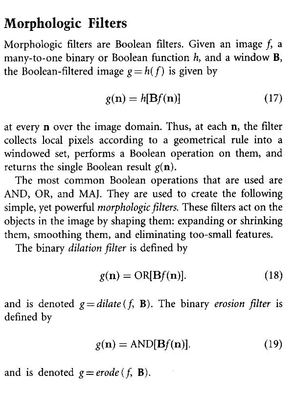
• Note that Bovik calls the binary median filter the majority filter, as the third morphological operation.
• Filippo Bergamasco from the University of Venice has a more modern Morphology lecture including gray-scale morphology, ending in the rice grains!
• Bovik 2005 has also a whole section (2.3) on Fourier Analysis. For instance, on page 58 Bovek gives both DSFT.
• I like their way of interpreting a FT: as a decomposition of an image in otrhonormal complex exponential basic functions.
• Another thing to note, is that if the spatial images are linear convolution, their DSFT also have convolutional relationship.
• I also like Figure 5:
  
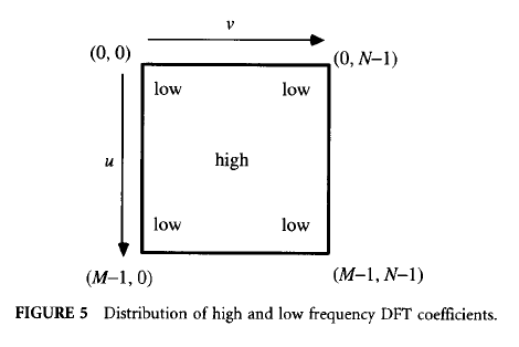
• Also great is section 2.3.5, Understanding DFTs. Such as
  • There is always a significant peak at origin, except when the image is dark.
  • An abundance of large coefficients near the origin indicates the existance of large and smooth image components (background).
  • Large objects like a collection of peppers give homogenious distrubuted low-frequency coefficients, while the edges contribute mid-to-higher frequenceies over a broad range of orientations.
  • When there a repeating patterns there are clear lines in the spectrum.

September 12, 2024

• Looked up the Robson-Campbell Curve. On the x-axis are the spatial frequency, on the y-axis the contrast:
  

September 9, 2024

• The color histogram slides I added from Linda Shapiro, were originally from Roger S Gaborski's lecture (2009). Couldn't find the original paper, although I found a nice histogram based face recognition PhD-thesis from CMU.
• I finished today at slide 79, so I didn't cover section 13.1.1 (shape from shading).
• Maybe I should add a small summary on Thursday, but I should check. Lecture 4 also has 135 slides, so it need to remove some content to make place.
• The slides should be better syncronized in the equation from the book and from the slides.
• For instance the slides as proportion between irradiance E^surface and radiance L^surface, while in eq. 2.84 it is the outcoming light is an integral of the incoming light times the BRDF, with the Phong shading a combination of three terms (ambient, diffuse, specular).
• Note that on slide 80, the specular spike/lob seems to be at the wrong side (specular: incoming = outcoming angle). The model of Torrance and Sparrow could matches with the specular lob of slide 80 (Gaussian?), with the specular spike corresponding to Phong's model (cos^ke). Yet, that depends on the variables.
• The material from this slides seems to come from here (or from the same source), but the slides don't match in style and concepts.
• Looking at Pong (1975). That is not the origin.
• I expect that the image on slide 80 should look like this:
  
• Note: only correct 'Diffuser'.
• An more modern (and simpler) figure can be found in Modeling outlier formation in scanning reflective surfaces using a laser stripe scanner (2014):
  
• At least these figures are accordance of Fig. 16 of Surface reflection: physical and geometrical perspectives (1991)
• Yet the figure in the slides is accordance of Fig. 17 of Surface reflection: physical and geometrical perspectives (1991)
   
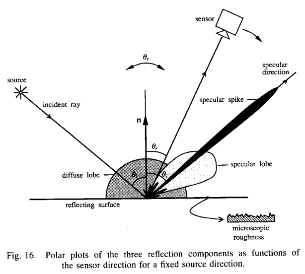
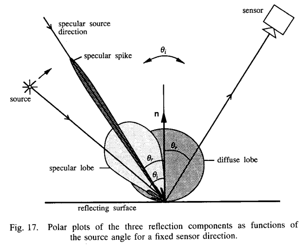
• The difference between Fig. 16 and 17 is what is fixed and what is varied. Fig. 17 (used in the slide 80) moves the source, because slide 79 indicates that in the Phong model the lighting direction is varied. Indeed, in Eq. (2.94) on page 57 the summation is on light source i, so Fig. 17 applies.
• Note that in a later paper Stereo and Specular Reflection they have a variant from Fig. 16 with 3 camera viewpoints (great for section 13.1.1), see Fig. 9a in that paper.
• They point back to Torrance and Sparrow's model (1967)
• Torrance and Sparrow use a 3D version of that drawing (without lobes):
  

September 6, 2024

• Watching the whole Relighting video is a bit long. After 1m27 (switch to previous work), or after 2m (end of previous work, I could jump to 7m07, where the highlights are explained. Could stop at 8m20, before we switch speakers to go deeper into the shading network.
• MIT intro concentrates on edges, so would be great for Lecture 4 / 5.
• For slide 37 / 78 I have seen a much higher resolution zebra. But where?
• Should look up what the Robson-Campell curve is about (left them out for the moment).

August 23, 2024

• Maybe I should add the Nvidia prisma image from this blog to the color slides, together with AAPS workflow.
• Figure 14-9 from Ray Tracing Gems II could be used in lecture 3

August 22, 2024

• Slide 5-7 of Joe Redmons' guest lecture on Color are nice for the 2nd lecture.
• Slide 32 nicely summarizes what color spaces means for computers.
• Also love slide 39, with how the geometric conversion between HSV and RGB.
• Also slide 40-47 is insightfull and fun.
• Looking for courses of the authors of Foundations.
• Phillip Isola was giving Advances in Computer Vision .
• For Antonio Torralba I could only find Deep Learning for AI and Computer Vision (professionals).
• William T Freeman gave in 2002 Machine Vision, in 2005 it was already renamed to Advances in Computer Vision.
• On the ICCV 2003 he gave a Course on Learning and Vision.
• The latest course information (2024) is here
• They claim to still using Szeliski's book, although I recognize their Foundation chapters. Looked into their Optical Flow slides (our 6th lecture). After explaining the classic approach with car at a Spanish road, they also cover state-of-the-art methods FlowNet (inspired by the classic approach).
• Also like that in MIT they have a AI assistant policy.
• Slide 12-15 of Lecture 4 nicely shows a classifier kernel.
• Slide 65 of handling boundaries (with a zebra) is also nice.
• Lecture 5 also highlights Hybrid images (slide 41-45).

August 21, 2024

• Requisted and received a (digital) evalution copy of Foundations of Computer Vision (2024).
• It has four chapters on Image Formation. I like Fig. 6.10, 6.11 and 6.12 for Depth of Field, the circle of confusion and apparture.
• Read 9.1, which actually has no illustration at all.
• For the filters, I love Figure 18.10 with a pyramid of Gaussian derivates up to order 6, with in Figure 18.11 the Fourier Transform.
• It actually has 4 chapters on motion, the topic of the 6th lecture.
• Like Fig. 46.5 on the effect of path-size on optical flow.
• Chapter 47 uses a geometrical approach, including ego-motion.
• Chapter 48 goes deeper into the algorithms to estimate optical flow, including Good features to track. Multiscale is impressive better (Fig. 48.10).
• Fig 1c is an illusion often used, 1b was new for me.
• Also love the Ibn al-Haytham as inverter of the Book of Optics, including Fig. 1.4.
• Also a lot of human perception, useable for BBR (section 1.3.3 and 1.3.4)
• There is also a whole section on Marr.

August 20, 2024

• The 5th lecture covers 7.2, 7.4 and 7.1.
• ORB and SURF features are not covered in the lecture, nor SuperPoint.
• A state-of-the-art algorithm is LightGlue
• LightGlue is cited in the 2024 paper DUSt3R: Geometric 3D Vision Made Easy.
• It is a bit overkill, but DUSt3R can be used for downstream tasks as estimating the focal length and relative position.
• The successor is called MASt3R.
• For color edges, they point to Theo Gevers' chapter Color Feature Detection (2006)
• Figure 1.1 is nice, because it reuses the luminance they encountered in the first assignment.
• Love slide 11 of Shapiro.
• Also the PCA on slide 31 from Lecture6 of Shapiro is good!
• The 6th lecture covers 9.1.1, 9.1.3 and 9.3.
• The 6th lecture is about optical flow, so I expect drones (check Scaramuzza).
• The local patch from Chapter 7 is presented in Lecture 6.
• Also the local descriptor images from Chapter 7 reappear.
• The 7th lecture of Martin overlaps with Lecture 7 of Shapiro.
• This trick worked to convert a ppsx to a pptx.

August 19, 2024

• The 4th lecture covers 3.2, 3.3 and 3.4.
• No idea why hybrid image was added to the slides (around slide 121).
• Read Oliva's paper for some background.
• Maybe nice to replace Prof. Pietro Perona image with All is vanity painting.
• Computer Vision is also given at University of Washingthon.
• The 4th lecture of Linda Shapiro (Filtering) should cover Szeliski 3.2 and 3.3.1
• Some of the basics (presented as side notes are covered by Shaodi.
• Shapiro is a completly different lecture, but with the 'standard' image from Yolo much more modern.
• This is 5-level course, there is also a 4-level course in Washingthon.
• Chapter 3.2 has whole section on integral image, where multiple box filters are combined. It would be nice to also give an example of that (pyramids, 2nd order derivates).
• Maybe make the link between averaging and max-pooling, and between interpolation and decimation with the resolution changes in decoder / encoder architectures.
• The first assignment comes together with Chapter 5 of Computer Vision: A Modern Approach (2012)
• That part is needed for the 4th part of the assignment, on Photometric stereo (section 5.4).
• Although I am running Ubuntu 20.04, my version of cv2, numpy and matplotlib is too modern. I am using cv2 4.2.0 instead of 3.4.8, numpy 1.24.4 instead of 1.19.5, matplotlib 3.7.4 instead of 3.3.4.
• I had already Xlaunch on my home-computer, I only need to add the PULSE_SERVER commands from this forum-post to setup X11 forwarding WLS2. Both xcalc and cv2.imshow() now works.
• Looking into OpenCV documentation for the actual conversion to gray scale.
• Solved rgb2grays assignment. Note to normalize the channels directly, otherwise you get overflow. Also note the difference between np.max() and np.maximum(), as indicated here.
• Check Wednesday if the lectures should be recorded.

August 18, 2024

• Slide 3 of Lecture 3 is confusing, the definitions don't match with the figure.
• The lecture covers 2.2.2, 3.1.1, 3.1.2, 3.1.4 and 13.1.1.
• After slide 11 (Geometric Operations), I could add Figure 2.4 with all possible Rigid Body transformation from Chapter 2.
• In Chapter 3, section 3.1.3 (Composition and Matting) is skipped.
• The Total Relighting movie from slide 40 is from ACM Transactions on Graphics July, 2021.
• Before going from Total Relighting to Surface normals et, would first recap Marr's four main factors: (1) the geometry and (2) the reflectances of the visible surfaces, (3) the illumination of the scene, and (4) the viewpoint.', maybe even illustrated with a NERF's model.
• Section 2.2.2 covers the BRDF model, no explicit mentioning of the Albedo model.
• Maybe good to remind that all these operations are the ones that actually performed during data augmentation, a method where you have most control off during training.
• Section 13.1 is Shape from X, with 13.1.1 Shape from Shadow. Should make this explicit in the slides, that we now encounter the first Shape from X application.
• The suggested further reading book of Ikeuchi (2020) mainly focuses on Active Lighting.

August 16, 2024

• Prof. Pietro Perona is from CalTech, and was on the basis of Merlin Bird ID.
• To be checked: Did Marr's book already distincted Low-, Medium- and High-level vision?
• The 2nd lecture concentrates on section 2.2 and 2.3. Yet, Figure 2.14 should be added to the slides, which covers all 4 aspects mentioned by Marr.
• It would be nice to add some Unreal Scenes, about ambient lighting and surface reflection.
• Should also show the photograph umbrella's.
• Slide 9 of this lecture has a nice example of anisotropic reflectance.
• Also slide 7 (four types of reflectance functions), is quite usefull.
• For more depth on the Image Formation, I could look at Brown's ICCV 2019 tutorial.
• Like his motivation: camera's are not reflectance measurement units, they produce visual pleasing photographs.
• Could reuse slide 26 (What is 'true blue')
• Love the Tristimulus color theory slide 34.
• It actually shows Harris's colour wheel.
• On this wikipedia page, the history of colour wheels is described, including Newton's original asymmetric color wheel based on musical intervals and Goethe's symmetric color wheel
• The flicker experiment at slides 38-40 where new to me.
• Also the negative component to CIE RGB color matching is new.
• Also love slide 59: the standard observers which devined colors where 17 participants.
• Also love slide 69, with the SPD of different outside conditions.
• Also slide 74 and 82,83 is usefull.
• Illuminant D is natural daylight, with different color temps (5000K, 5500K, 6500K), which makes up the illumination D50, D55, D65.
• Combined with slide 88 (each device is different) and the sRGB white point (depedent on D50 and D65). Result on slide 95.
• Note that CIE XYZ is the mother of all color spaces (slide 99)
• Part II is on the pipeline. Slide 122 is important: the pixel is a relative digital value.
• Also slide 127 is nice, with the dead pixel interpolation.
• Slide 183 indicates why this knowledge is important. Certain CV algorithms assume linear response to physical light, which is only true for raw-RGB. All image from the web are sRGB. See slide 185 shows the effect on deblurring.

August 15, 2024

• Until week 39, there are 6 lectures to be covered (Monday and Thursday afternoon, in C1.110 and L1.02)
• The basis of the course is Szeliski 's book Computer Vision.
• Ordered a softcover of the book.
• The following topics are covered in the first six lectures:
  • Camera geometry
  • Image formation and Color
  • In place processing, Reflection model, Photometric Stereo, Shape from X
  • Neighbourhood Processing, Image Filtering
  • Neighborhood operations, image filtering
  • Edges and corners
• In principal, I need to read Chapter 1-3, 7 and 9.
• Szeliski's book is also used in Computer Vision 1 and Computer Vision 2.
• Structure from motion and SLAM is covered in the 3rd lecture of CV2.
• Chapter 12 Depth Estimation, is not covered by CV2.
• The last chapter of Szeliski is Image-Based rendering, which is also not explicit covered in CV2.
• Chapter 8 - Image Alignment and Stitching and Chapter 9 - Motion Estimation will be covered in Vision for Autonomous Robots. No idea if this is covered in CV1.
• Went to the first 111 slides of the first lecture. Because the logistics is explained, many slides have to be updated.
• Should look at David Marr's book Vision (MIT Press, 2010 - reprint of the 1982 original), because it is mentioned several times in the first lecture. (432 pages). The book is also mentioned by Szeliski at page 11, point for more recent developments to (Wandell 1995, Palmer 1999m, Livingstone 2008 and Frisby and Stone 2010). Should snowball the last publication.
• A lot of the week 3 topics where first covered in the 1980s.
• Finished Chapter 1 of Szeliski's book.
• Read the first chapter of Marr's book.
• In Marr's 2nd chapter he claims ' There are four main factors responsible for the intensity values in an image. They are (1) the geometry and (2) the reflectances of the visible surfaces, (3) the illumination of the scene, and (4) the viewpoint.'. He formulates the (2 1/2 D) sketch as a reconstruction in a viewer-centered coordinate frae. Read most of section 2.2, I still have to look at 2.3 (Spatial Arrangement), 2.4 (Light sources and Transparency), 2.5 (Grouping process and full primal sketch).
• I also should do the first three tutorials.

Previous Labbooks