Jan van Eijck
Sept 20, 2016
> module FSA3 where
>
> import FSA2 (while,whiler)
Overview
While Loops as Fixpoints
The definition of a fixpoint operation.
> fp :: Eq a => (a -> a) -> a -> a
> fp f = until (\ x -> x == f x) f
Using this, we can construct another variation on Fibonacci:
> fbo n = fibo (0,1,n) where
> fibo = fp (\ (x,y,k) -> if k == 0 then (x,y,k)
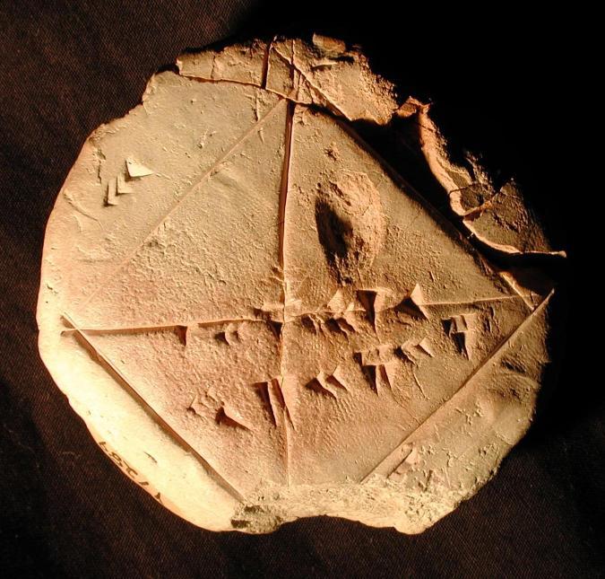
> else (y,x+y,k-1))YBC7289: Approximating \(\sqrt{2}\)
The Babylonian method of computing square roots: repeatedly take the average of an overestimation \(x\) and an underestimation \(a/x\) to \(\sqrt{a}\).
If \(\sqrt{a} < x\) then \(a/\sqrt{a} > a/x\), i.e., \(a/x < \sqrt{a}\).
Conversely, if \(\sqrt{a} > x\) then \(a/\sqrt{a} < a/x\), i.e., \(a/x > \sqrt{a}\).
Next, take the average of \(x\) and \(a/x\).
That is, consider the function \(\lambda x \mapsto \frac{x +a/x}{2}\).
Let \(y\) be a fixpoint of \(\lambda x \mapsto \frac{x +a/x}{2}\).
Then
\(y = \frac{y +a/y}{2}\)
\(2y = y +a/y\)
\(y = a/y\)
\(y^2 = a\)
\(y = \sqrt{a}\)
This works well in Haskell because of the limited precision of floating point numbers.
> bab a = \ x -> ((x + a/x)/2)
>
> sr a = fp (bab a) a
This gives:
 *FSA3> sr 2
 1.414213562373095
 *FSA3> sr 3
 1.7320508075688772
 *FSA3> sr 4
 2.0
 *FSA3> sr 5
 2.23606797749979
Review question How can you test this square root program?
To see a bit clearer what goes on here, use the following function:
> iterateFix :: Eq a => (a -> a) -> a -> [a]
> iterateFix f = apprx . iterate f where
>   apprx (x:y:zs) = if x == y then [x] else x: apprx (y:zs)
*FSA3> iterateFix (bab 2) 1
[1.0,1.5,1.4166666666666665,1.4142156862745097,1.4142135623746899,1.414213562373095]
*FSA3> iterateFix (bab 3) 1
[1.0,2.0,1.75,1.7321428571428572,1.7320508100147274,1.7320508075688772]
*FSA3> iterateFix (bab 4) 1
[1.0,2.5,2.05,2.000609756097561,2.0000000929222947,2.000000000000002,2.0]Fix
Haskell has a special fixpoint operator that can be used to implement recursion.
> fix :: (a -> a) -> a
> fix f = f (fix f)
Alternative definition:
fix f = let x = f x in x> fbx n = fibo (0,1,n) where
> fibo = fix (\ f (x,y,k) -> if k == 0 then (x,y,k)
> else f (y,x+y,k-1))Without using fix:
> fbb n = fbbb (0,1,n) where
>   fbbb (x,y,n) = if n == 0 then x else fbbb (y,x+y,n-1)
Or in curried notation:
> fbc n = fbbc 0 1 n where
>   fbbc x y n = if n == 0 then x else fbbc y (x+y) (n-1)
Fix can be used to implement recursion without using other functions that call themselves.
To see why this works, notice that fbx will compute a fixed point of the function
  k = (\ f (x,y,k) ->
        if k == 0 then (x,y,k) else f (y,x+y,k-1))
that is, a function h such that h = k h:
  h = k h =
     (\ f (x,y,k) ->
        if k == 0 then (x,y,k) else f (y,x+y,k-1)) h
    = \ (x,y,k) ->
        if k == 0 then (x,y,k) else h (y,x+y,k-1))
This is indeed the recursive Fibonacci function.
Review question
Explain the connection between fp and fix.
To see a connection between fp and fix, consider the following definition of fp in terms of fix:
> fp' :: Eq a => (a -> a) -> a -> a
> fp' f = fix (\ g x -> if x == f x then x else g (f x))
And here are definitions of until and while in terms of fix:
> until' :: (a -> Bool) -> (a -> a) -> a -> a
> until' p f = fix (\ g x -> if p x then x else g (f x))
> while' :: (a -> Bool) -> (a -> a) -> a -> a
> while' p f = fix (\ g x -> if not (p x) then x else g (f x))Reasoning about Functions
One way to think about a function is as an assignment of values to some objects of a certain type.
In mathematics, \(f : A \to B\) expresses that \(f\) is a total function from \(A\) to \(B\), i.e., for every \(x \in A\) there is an \(fx \in B\).
For example a function \(f : {\mathbb Z} \to {\mathbb Z}\) can be identified with its graph. (\(\mathbb Z\) is the set of integer numbers, from the German Zahlen.)
I.e., \(f : {\mathbb Z} \to {\mathbb Z}\) can be thought of as the infinite set of pairs given by: \(\{ (x,fx) \mid x \in {\mathbb Z} \}\). This does not quite match the situation in functional programming.
f :: a -> b does declare f as a function from objects of type a to objects of type b, but there is no assumption that this function is total.
Thinking about the class of partial functions from objects of type a to objects of type b, there is an obvious information order on them. Let us use \(f x = \bot\) for $f x$ is undefined. It follows that \(f x \neq \bot\) expresses that \(f x\) is defined.
We start with a partial order on basic types. For any basic type \(a\), we introduce an object \(\bot :: a\) for the undefined object of that type, and we define an ordering on the type by means of
\[ x \sqsubseteq y \text{ if } x = \bot \lor x = y. \]
Thus, if \(u\) and \(v\) are two objects of type \(a\) that are different from \(\bot\) and from each other, then this ordering is given by:
\[ \sqsubseteq \ = \{ (\bot, \bot), (\bot, u), (\bot, v), (u,u), (v,v) \}. \]
Haskell uses undefined for \(\bot\).
For the particular case of the Booleans, we have:
\[ \sqsubseteq \ = \{ (\bot, \bot), (\bot, T), (\bot, F), (T,T), (F,F) \}. \]
Partial Orders and Strict Partial Orders
A binary relation on a set \(X\) is a subset of \(X^2\), where \(X^2\) is the set of all pairs of elements taken from \(X\).
A binary relation \(R\) on \(X\) is called a partial order if \(R\) is transitive \((\forall x y z ((Rxy \land Ryz) \rightarrow Rxz)\), reflexive (\(\forall x Rxx\)) and antisymmetric (\(\forall x y ((Rxy \land Ryx) \rightarrow x = y)\).
A binary relation \(R\) on \(X\) is a strict partial order if \(R\) is transitive and irreflexive (\(\forall x \neg Rxx\)).
Every partial order \(R\) contains a strict partial order \(S\) given by \(Sxy := Rxy \land x \neq y\).
The strict partial order \(\sqsubset\) corresponding to \(\sqsubseteq\), on the Booleans, is given by:
\[ \sqsubset \ = \{ (\bot, T), (\bot, F) \}. \]
The strict partial order \(\sqsubset\) corresponding to \(\sqsubseteq\), on the integers, is given by:
\[ \sqsubset \ = \{ \ldots, (\bot, -2), (\bot, -1), (\bot, 0), (\bot, 1), (\bot, 2), \ldots \}. \]
Next, we lift these orderings on basic types to functional types.
Let \(P = A \hookrightarrow B\) be the set of all partial functions from \(A\) to \(B\).
We define a binary relation \(\sqsubseteq\) on \(P\) by stipulating:
\[ f \sqsubseteq g \text{ iff } \forall x : \text{ if } x \neq \bot \land f x \neq \bot \text{ then } f x = g x. \]
Monotonicity
Note that \(f x \neq \bot\) expresses that \(f\) is defined on \(x\). We exclude the situation where \(x = \bot\) and \(f x\) is defined. In other words, we expect our partial functions to be monotonic for the information order \(\sqsubseteq\).
A function \(f\) is monotonic for \(\sqsubseteq\) if \(x \sqsubseteq y\) holds iff \(fx \sqsubseteq fy\) holds.
Meet of two functions
Use \(f \sqcap g\) for the function \(h\) given by:
\[ h x = \left\{ \begin{array}{cc} f x & \text{ if } f x = g x \\ \bot & \text{ otherwise } \end{array} \right. \]
The function \(f \sqcap g\) is called the greatest lower bound or meet of \(f\) and \(g\).
We say that partial functions in \(A \to B\) are a meet semilattice for the partial order \(\sqsubseteq\). For every pair of functions \(f\) and \(g\) with domain \(A\) and codomain \(B\), their meet \(f \sqcap g\) is defined. Moreover, \(f \sqcap g\) is the largest function \(h\) in the \(\sqsubseteq\) order that satisfies \(h \sqsubseteq f\) and \(h \sqsubseteq g\).
Join of two functions
Let \(f\) and \(g\) be such that for all \(x\) with \(f\) and \(g\) both defined for \(x\) it holds that \(f x = g x\). If this is the case we can define the least upper bound or join of \(f\) and \(g\), notation \(f \sqcup g\), as the function \(h\) given by:
\[ h x = \left\{ \begin{array}{cl} f x & \text{ if } f x \neq \bot \\ g x & \text{ if } f x = \bot \text{ and } g x \neq \bot \\ \bot & \text{ otherwise } \end{array} \right. \]
Consider the following built-in function for iterating an operator \(f\) starting from a given value \(x\):
iterate :: (a -> a) -> a -> [a]
iterate f x = x: iterate f (f x)
Use for constructing a list of functions starting from \(\bot\), ordered by \(\sqsubset\), and approximating the factorial function:
> apprFact :: (Integer -> Integer) -> Integer -> Integer
> apprFact = \ f n -> if n == 0 then 1 else n * f (n-1)
Now consider the sequence \(f_0, f_1, f_2, \ldots\) given by:
f0:f1:f2:f3:f4:f5:f6:fs = iterate apprFact undefinedThen \(\bot = f_0 \sqsubset f_1 \sqsubset f_2 \sqsubset f_3 \sqsubset f_4 \sqsubset f_5 \sqsubset \cdots\)
 *FSA3> f1 0
 1
 *FSA3> f1 1
 *** Exception: Prelude.undefined
 *FSA3> f2 1
 1
 *FSA3> f2 2
 *** Exception: Prelude.undefined
 *FSA3> f3 2
 2
 *FSA3> f3 3
 *** Exception: Prelude.undefined
 *FSA3> f4 3
 6
The functions in the series are all approximations of the factorial function, with the domain of definition of \(f_n\) equal to \(\{ 0, \ldots, n-1 \}\).
The factorial function is the least fixpoint of this series of approximations:
> fact = fix apprFactLet \(P = A \hookrightarrow B\). As we have seen, the ordering \(\sqsubset\) on the set \(P\) is a strict partial order, and also a meet semilattice. It is not a lattice, for binary joins \(f \sqcup g\) may not exist for \(f,g \in P\).
The partial order \(\sqsubseteq\) is complete, in the following sense. If \(F \subseteq P\) then let
\[ F^u := \{ g \mid \forall f \in F: f \sqsubseteq g \}. \]
Thus, \(F^u\) consists of all upper bounds of \(F\): all functions that are above any \(f \in F\) in the \(\sqsubseteq\) ordering.
Directedness
A subset \(S\) of \(P\) is called directed if for every finite \(F \subseteq S\) there is an \(f \in S\) with \(f \in F^u\), i.e., \(S\) is directed if every finite subset of \(S\) has an upper bound in \(S\).
Example
The set \(\{ f_i \mid i \in {\mathbb N} \} \subseteq {\mathbb N} \hookrightarrow {\mathbb N}\) (the set of approximations to the factorial function) is an example of a directed set.
Least Upper Bound
A least upper bound of \(S\) is a member of \(S^u\) that is below any member of \(S^u\) in the \(\sqsubseteq\) ordering. If \(S\) has a least upper bound, we refer to it as \(\sqcup S\).
Completeness of \(P = A \hookrightarrow B\) means:
The set \(P\) has a bottom element \(\bot\), namely the function that is everywhere undefined.
If \(S\) is a directed subset of \(P\) then \(\sqcup S\) exists.
The set \(P = A \hookrightarrow B\), partially ordered by \(\sqsubseteq\), is complete. For further information on this lattice-theoretic perspective on spaces of partial functions see (Davey and Priestley 2002).
Specification Assertions as Wrappers
One way to write assertions for functional code is as wrappers around functions. This results in a much stronger sense of self-testing than what is called self-testing code (code with built-in tests) in test driven development (Beck 2002).
The precondition of a function is a condition on its input parameter(s), the postcondition is a condition on its value.
Precondion wrapper for functions with one argument.
The wrapper takes a precondition property and a function and produces a new function that behaves as the old one, provided the precondition is satisfied,
> pre :: (a -> Bool) -> (a -> b) -> a -> b
> pre p f x = if p x then f x else error "pre"
Postcondition wrapper for functions with one argument.
> post :: (b -> Bool) -> (a -> b) -> a -> b
> post p f x = if p (f x) then f x else error "post"
This can be used to specify the expected outcome of a function.
Consider the following example:
> decomp :: Integer -> (Integer,Integer)
> decomp n = decmp (0,n) where
>   decmp = until (odd.snd) (\ (m,k) -> (m+1,div k 2))
The purpose of this is to factor out powers of \(2\). A formal specification of the expected outcome is given by:
> decompPost :: Integer -> (Integer,Integer)
> decompPost = \n -> post (\ (m,k) -> 2^m * k == n) decomp n
This specifies that the output \((m,k)\) for input \(n\) should satisfy \(2^m \cdot k = n\).
Note that decompPost has the same type as decomp, and that the two functions compute the same value whenever decompPost is defined, i.e., whenever the output value of g satisfies the postcondition.
More generally, an assertion is a condition that may relate input parameters to the computed value. A assertion wrapper wraps a binary relation expressing a condition on input and output around a function and produces a new function that behaves as the old one, provided that the relation holds.
> assert :: (a -> b -> Bool) -> (a -> b) -> a -> b
> assert p f x = if p x (f x) then f x else error "assert"
Example use:
> decompA :: Integer -> (Integer,Integer)
> decompA = assert (\ n (m,k) -> 2^m * k == n) decomp
Note that decompA has the same type as decomp. Indeed, as long as the assertion holds, decompA and decomp compute the same value.
We can also use an assertion to check the step function inside decomp:
> stepA :: (Integer, Integer) ->  (Integer, Integer)
> stepA = assert (\ (m,k) (m',k') -> 2^m*k == 2^m'*k')
>                 (\ (m,k) -> (m+1,div k 2))
Invariants
An invariant of a program \(P\) in a state \(s\) is a condition \(C\) with the property that if \(C\) holds in \(s\) then \(C\) will also hold in any state that results from execution of \(P\) in \(s\). Thus, invariants are Hoare assertions of the form:
\[ \{ \text{C} \} \ \text{Program} \ \{ \text{C} \} \]
If you wrap an invariant around a step function in a loop, the invariant documents the expected behaviour of the loop.
First an invariant wrapper for the case of a function with a single parameter: a function fails an invariant if the input of the function satisfies \(p\) but the output does not:
> invar :: (a -> Bool) -> (a -> a) -> a -> a
> invar p f x =
>   let
>     x' = f x
>   in
>    if p x && not (p x') then error "invar" else x'
Examples:
> succI = invar (>0) succ
>
> predI = invar (<0) pred
We can also use the invariant to check a step function inside a while loop:
> largestOddFactor = while even (invar (>0) (`div` 2))Any call to a function with a precondition, postcondition, assertion or invariant wrapped around it tests the specification of the function.
Example:
> predI' = invar (>0) predExample use:
 *FSA3> predI 1
 0
 *FSA3> predI' 1
 *** Exception: invar
The Extended GCD Algorithm
The extended GCD algoritm extends the Euclidean algorithm, as follows. Instead of finding the GCD of two (positive) integers \(M\) and \(N\) it finds two integers \(x\) and \(y\) satisfying the so-called Bézout identity (or: Bézout equality):
\[ xM + yN = \gcd(M,N). \]
For example, for arguments \(M = 12\) and \(N = 26\), the extended GCD algorithm gives the pair \(x = -2\) and \(y = 1\). And indeed, \(-2 * 12 + 26 = 2\), which is the GCD of \(12\) and \(26\).
GCD Lemma
If \(D \mid M\) and \(D \mid N\) and \(D = xM + yN\) (with \(x,y \in {\mathbb Z}\)), then \(D = \gcd(M,N)\).
Proof
From \(D \mid M\) and \(D \mid N\) we get that \(D \leq \gcd(M,N)\).
From \(\gcd(M,N) \mid xM\) and \(\gcd(M,N) \mid yN\) it follows that \(\gcd(M,N) \mid xM + yN\), i.e., \(\gcd(M,N) \mid D\). Therefore, \(\gcd(M,N) \leq D\).
Combining (1) and (2) we get \(\gcd(M,N) = D\). QED
What the GCD Lemma tells us is that if we can find \(x\) and \(y\) with the property that \(xM + yN\) divides both \(M\) and \(N\) then we know that we have found the GCD of \(M\) and \(N\). The following algorithm (iterative version) accomplishes this:
Let positive integers \(a\) and \(b\) be given.
A proof of the correctness of this algorithm is given in Section 8.2 of (Doets and Eijck 2012).
The mathematical importance of the extended GCD Algorithm is that it is the key to the fundamental theorem of arithmetic:
Fundamental Theorem of Arithmetic
Every natural number greater than \(1\) has a unique prime factorization.
The practical importance of extended GCD Algorithm is that it is a building block for the RSA algorithm for public key cryptography.
Functional imperative version of the extended GCD algorithm, in Haskell:
> ext_gcd :: Integer -> Integer -> (Integer,Integer)
> ext_gcd a b = ext_gcd' (a,b,0,1,1,0) where
>     ext_gcd' = whiler
>                  (\ (_,b,_,_,_,_) ->  b /= 0)
>                  (\ (a,b,x,y,lastx,lasty) -> let
>                     (q,r)   = quotRem a b
>                     (x',lastx') = (lastx-q*x,x)
>                     (y',lasty') = (lasty-q*y,y)
>                  in (b,r,x',y',lastx',lasty'))
>                  (\ (_,_,_,_,lx,ly) -> (lx,ly))
Bézout's identity is turned into an assertion, as follows:
> bezout :: Integer -> Integer -> (Integer,Integer) -> Bool
> bezout m n (x,y) = x*m + y*n == euclid m n
> euclid m n = fst $ eucl (m,n) where
> eucl = until (uncurry (==))
> (\ (x,y) -> if x > y then (x-y,x) else (x,y-x))Use this to produce assertive code for the extended algorithm:
> ext_gcdA = assert2 bezout ext_gcdThis uses an assertion wrapper for functions with two parameters:
> assert2 ::  (a -> b -> c -> Bool)
>              -> (a -> b -> c) -> a -> b -> c
> assert2 p f x y =
>   if p x y (f x y) then f x y
>   else error "assert2"
A functional (recursive) version of the extended Euclidean algorithm:
> fct_gcd :: Integer -> Integer -> (Integer,Integer)
> fct_gcd a b =
>   if b == 0
>   then (1,0)
>   else
>      let
>        (q,r) = quotRem a b
>        (s,t) = fct_gcd b r
>      in (t, s - q*t)
Again, an assertive version of this:
> fct_gcdA = assert2 bezout fct_gcdStill, proofs are better than tests, and the recursive version of the extended Euclidean algorithm allows an inductive correctness proof.
The functional version of the extended Euclidean algorithm is correct, for all non-negative arguments.
Assertive Code is Efficient Self-Documenting Code
More often than not, an assertive version of a function is much less efficient than the regular version: the assertions are inefficient specification algorithms to test the behaviour of efficient functions.
But this does not matter. To turn assertive code into self-documenting production code, all you have to do is load a module with alternative definitions of the assertion and invariant wrappers.
Take the definition of assert. This is replaced by:
 assert :: (a -> b -> Bool) -> (a -> b) -> a -> b
 assert _ = id
The assertions are still in the code, but instead of being executed they now serve as documentation. The assertive version of a function executes exactly as the version without the assertion.
Assertive code comes with absolutely no efficiency penalty.
What are we testing?
Suppose a program (implemented function) fails its implemented assertion. What should we conclude? This is a pertinent question, for the assertion itself is a piece of code too, in the same programming language as the function that we want to test.
So what are we testing, the correctness of the code or the correctness of the implememented specification for the code?
In fact, we are testing both at the same time. Therefore, the failure of a test can mean either of two things, and we should be careful to find out wat our situation is:
In both cases it is important to find out where the problem resides. In the first case, we have to fix a code defect, and we are in a good position to do so because we have the specification as a yardstick. In the second case, we are not ready to fix code defects. First and foremost, we have to fix a defect in our understanding of what our program is supposed to do. Without that growth in understanding, it will be very hard indeed to detect and fix possible defects in the code itself.
How to Integrate Implementation and Specification
State-of-the-art functional programming languages are well suited not only for implementing algorithms but also for specifying algorithms and wrap the specifications around the implementations, to produce assertive code.
In fact you can do this with any language, but the cost is higher (sometimes much higher) for less abstract languages.
Functional Imperative Programming
We have seen that imperative algorithms can be implemented directly in a functional language. The while loops that were employed above are explicit about the parameters that are used for checking loop termination and for defining the loop step. This often makes the implemented algorithms more perspicuous.
Beck, Kent. 2002. Test Driven Development by Example. Boston, MA: Addison-Wesley Longman.
Davey, B.A., and H.A. Priestley. 2002. Introduction to Lattices and Order (Second Edition). Cambridge University Press, Cambridge.
Doets, K., and J. van Eijck. 2012. The Haskell Road to Logic, Maths and Programming, Second Edition. Vol. 4. Texts in Computing. London: College Publications.