Quantitative associations: ANOVA
This lab treats the statistical methodology of the analysis of variance. You can start by loading LAB5.mat and making an .m file (script) for your own answers. Before you start, fill in your name, student number and the date in the header of your script. Name your script as follows: YourName_LAB5.m
Contents
Hypothesis testing and the ANOVA
An ANalysis Of VAriance or ANOVA allows the comparison of several means of several groups. An ANOVA is often used when you deal with more than 2 groups. In this lab we use the symbol g for the number of groups. The symbols  ,
,  and
and  denote the population means of the various groups.
Before we move on, to the technical details of an ANOVA, let's first get our hypotheses right. Choose the most appropriate set of hypotheses for an ANOVA.
- H0:
 >
>  =
=  , H1: at least two population means are unequal
 - H0:
 =
=  =
=  , H1: all population means are unequal.
 - H0:
 =
=  =
=  , H1: at least two population means are unequal.
ANOVA and Types of variance
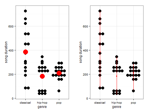
The reason why an analysis of variance is called an analysis of variance is that we compare two different types of variances. Essentially we test the ratio of between group and within group variance. Let's consider visually what this means. To do so, we use a subset of data from the 1 million song dataset retrieved from the following link: "http://labrosa.ee.columbia.edu/millionsong/blog/11-2-28-deriving-genre-dataset" The table songdata (in LAB5.mat) gives the length of songs (duration in seconds) for three different music categories. And the table songdata2 adds information about the geographical origin (Europe or North America) to the set.

On the left-most visualization, the big red dots represent the group averages. As you can see, there are some differences in the average song duration per genre. The differences between the group averages form the basis for the between-group averages. On the right most visualization, the red lines give an idea of the varition within groups. As you see, for this sample of songs, the song duration of classical songs range from approximately 100 seconds to a little over 700 seconds. Based on each individual observation, the witin-group variance (i.e. the variance within each genre) is calculated).
The larger the between-group variance relative to the within-group variance, the more variance is explained using the groups means. Therefore, the better the seperate means can explain the variance in the data. In turn, this results in a larger F statistic. Before we continue to calculate our F statistic, let's first calculate some useful summary statistics. Our data are stored in a "table". You can use dot-indexing to access columns (e.g. data.names or data.times).
- Calculate the overall average song duration and store it in a variable called `grand_mean`. The overall data is available in a table called `songdata`.
- Save the duration of the claasical, hip-hop, and pop songs in seperate data structures (there are multiple ways to do this).
- Calculate the average song duration for the classical genre and store it in a variable called `classical_average`. Create a subset of only data for classical songs youself.
- Calculate the average song duration for the hip hop genre and store it in a variable called `hiphop_average`.
- Calculate the average song duration for the pop genre and store it in a variable called `pop_average`.
Calculating the Between Group Variance
Now that we've got our grand mean and the means of the different genres, we can calculate the between group variance. The formula for the between group variance is the following: 
Okay, this formula looks really complicated so let's chop it up into parts. n here represents the sample size, so  represents the sample size of group 1 while
  represents the sample size of gth group. In our current example, we only have three different genres and thus three different groups so this formula would go up
  .
.  represents the average of group 1.
  would represent our overall average which is available in the variable `grand_mean`. g here represents the number of groups.
In the current exercise our overall average is stored in the console in the variable `grand_mean` while our group averages are stored in the variables `classical_average`, `hiphop_average` and `pop_average`. You should still have the data of the duration per genre from the previous question.
- Calculate the sample size of each group. Store the sample size of the classical genre in the variable called `nclassic`, the sample size of hip hop genre in the variable called `nhiphop` and the sample size of the pop genre in the variable `npop`.
- Calculate the between group variance per genre and store it in a variable called `between_group_var`.
Calculating Within Group Variance
Now that we've got our grand mean and the means of the different genres and our between group variance, we continue to calculate our within group variance. The formula for the within group variance is the following: 
Again this formula looks complicated so let's chop it up into parts.  represents each observation in a group and
  represents the mean for that group. What we then do is that we subtract the group mean from each group observation, square this and then sum it. If we are done with the first group, we repeat this procedure for the second group and so on. The total sum of this procedure, which is called the within sum of squares, is then divided by the total sample size (N) - the number of groups (g). The result is the within group variance.
- Calculate the sums of squares of the classical genre and save it in `sum_squares_classical`, do the same for the other genres.
- Add the within sum of squares for every group together and divide this by the
 . Store the result in the variable `within_group_variance`.
Calculating the F-statistic
Now that we have calculated the between-group and the within-group variance, we can calculate its ratio. The ratio of between-group and within-group variance produces a F statistic. See the following formula: 
An F statistic will become larger if the between-group variance rises and the within-group variance stays the same. The F statistic will become smaller if the within-group variance becomes larger and the between-group variance stays the same. The F statistic has a F sampling distribution. This distribution is approximately centered around F = 1 when the null hypothesis is true. The larger the F statistic, the stronger the evidence against the null hypothesis.
The F distribution has two different degrees of freedom: df1 and df2. The formula for df1 is the following:  where g is the amount of groups. The formula for df2 is the following:
  where N is the sample size of all groups combined and g is the number of groups. These degrees of freedom come in handy when we want to calculate a p value for our obtained F statistic. To calculate a p value for our F statistic, we can use the `fcdf()` function. This function works similarly as the `tcdf()` and other cdf-functions that you may have come across in this and previous courses. The `fcdf()` function takes our F statistic as its first argument, our df1 as its second argument and our df2 as its third argument:
- The variables `between_group_variance` and `within_group_variance` are available in your console. Use these variables to calculate the F statistic and store the result in a variable called `f_stat`.
- Calculate the degrees of freedom df1 and df2 and store them in the variables `df1` and `df2`.
- Using the `fcdf()` function, calculate the p value and store this in the variable `p_value`. Make sure to calculate the p value associated with the upper tail.
Checking assumptions of ANOVA
As you may recall from the videos, there are three important assumptions that need to be checked before doing an analysis of variance:
- The population distribution for the dependent variable for each of the g groups need to be approximately normal
- Those distributions for each of the groups have the same standard deviation (homogeneity of variances)
- The data resulted from random sampling
In this exercise we are going to check the for the first two assumptions. To check for normality in each of our different genres, we are going to use the MatLab function `lillietest()`. You can give this function a vector of numeric values from a group. For instance, we can provide it our duration variable, like so: `classicaldata.duration`. This will test the null hypothesis the data comes from a normal distribution.
To check whether each group approximately has the same standard deviation, we are going to use the MatLab Levene's test. This test has been implemented in the `vartestn()` function. You use it like this: vartestn(dependent variable, variable of groups, 'TestType', 'LeveneAbsolute'). This will test the null hypothesis the variances of the groups are equal.
- Check whether the data points of the classical genre are approximately normally distributed. Do the same test for the hip hop and pop genre data. Note that when the "h" output of lillietest(x) is 0, this indicates that the null hypothesis - the data in vector x comes from a normal distriubtion - is not rejected. This implies that the assumption of normality is met. Note that we cannot say "the data comes from a normal distribution", as this is the same as accepting the null-hypothesis. For each sample, is the assumption of normality violated or not?
- Check for homogeneity of variance using the Levene's test. The combined data is available in the `songdata` table. The null hypothesis of this test is that the data comes from populations with equal variances. Is the assumption violated?
Explaining the ANOVA Function
In the last exercise we saw that both our assumption of normality and the assumption of homogeneity of variance were not met. Usually this would mean that we would perform a non-parametric test. These tests will be illustrated during the next week. However, during this lab we will continue to do an analysis of variance and will interpret the output as though our assumptions are met.
In MatLab there are two ways to perform an analysis of variance: the `anova()` functions (like `anova1()`, `anovan()`, etc.) and the `fitlm()` function. For now we will use the `anova1()`. There are only minor differences between the different functions - mainly in the way the output is presented. The anova1() and anovan() functions produce a more traditional ANOVA output.
- Peform an ANOVA using the `anova1()` function with genre as the independent variable and song duration as the dependent variable. If y is your dependent variable and x is your independent variable, you could perform an ANOVA through the following command: `anova1(y, x)`. Store the p, tbl and stats outputs from the ANOVA.
- Perform an ANOVA using the `fitlm()` function with genre as independent variable and song duration as the dependent variable. Store the result in a variable called `mdl_anova`. The easiest way to do this is by using the 'equation notation' in fitlm for this ( fitlm(DataTable,'your model-equation') ). If you would use the 'matrix notation' ( fitlm(Predict-matrix,response-vector) ), you first have to convert the predictor vector to a categorical variable.
Interpreting the output from an ANOVA
In the last exercise we produced output from the `anova1()` function. Inspect the `tbl` object to check whether we can reject the null hypothesis. The p value is in the `Prob>F` column. What does this p value mean in the context of the current data?
- This means that there is a difference in song duration for the classical and hip hop genre.
- This means that there is no difference in song duration for any of the genres
- This means that there is a difference in song duration for the different genres. However, we don't know yet which genres differ significantly from each other.
ANOVA: Multiple comparisons
An ANOVA checks for an overall difference in groups, i.e. you know that at least two groups differ from each other, but you don't know which groups. Under most circumstances you would therefore like to follow up an ANOVA with one or multiple post-hoc analyses. However, one has to be careful to control the family-wise error rate when following up an ANOVA with multiple post hoc analyses.
The family-wise error rate is the probability of making a type 1 error. Normally our type 1 error rate is denoted by  which we usually keep at 0.05. This means that there is a 5% chance of falsely rejecting the null hypothesis. E.g. We would conclude there is a difference between groups while there is none. If we have 5 different groups and we want to test whether every average differs from every other average with t-tests, we would need 10 tests. This would increase our family-wise error rate. This is because for each individual test we do, there is a 5% chance that we falsely reject the null hypothesis and this adds up. If we don't control for multiple testing, the family-wise error rate
  where m is the number of tests that we do.
To do 10 t-tests all with a significance level  of 5%, what would be our family-wise error rate? Use the formula displayed above and fill in the gaps. What does this family-wise error rate mean in this context?
- The family-wise error rate becomes 40%. This means that there's a probability of 0.4 that we falsely reject at least 1 null hypothesis.
- The family-wise error rate stays 5%. This means that there's a probability of 0.05 that we falsely reject at least 1 null hypothesis.
- The family-wise error rate becomes 40%. This means that there's a probability of 0.4 that we falsely reject all null hypotheses.
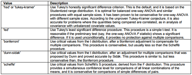
In MatLab a handy function to follow up an ANOVA with pairwise comparisons is the multcompare(stats) procedure. It is time to take a look at exactly what this function does. Apart from 'stats' in can accept two additional parameters; 'alpha' and 'ctype'. Your multiple comparison function will look like this: multcompare(stats, 'alpha', 0.05, 'ctype', 'hsd'). Ctype specifies which post-hoc test should be used. There's a variety of possible tests to perfom, each of which is preferable under specific conditions. The table below lists the possible values of the 'ctype' argument:

- Use the `multcompare()` function to follow-up your ANOVA analyses and print the output to the console. Make sure to calculate 'stats' first. All variables are available in the `song_data` dataframe. The output of multcompare is an array of pairwise comparisons (first two columns indicate group numbers which are comapred) and differences among groups (column 3 to 5 represent lower CI, mean and upper CI for the difference between the two groups) and a p value (last row).
- Perform the 'tukey-kramer' and 'bonferroni' post-hoc tests, print the output to the console and briefly discuss the main differences.
- By specifying he option 'lsd' for the input parameter 'ctype', multcompare() calculates the differences between groups through (uncorrected) independent t-tests. Apply this option als well and compare the results with those from the tukey-kramer option.
Two-way ANOVA
A two-way ANOVA is used when you want to compare multiple groups across multiple independent variables. To make our dataset suitable for a two-way ANOVA, we have added a new variable called "continent". This variable indicates whether the song was produced in North America or in Europe. Note that this variable has been simulated and was not available in the original datset.
Before we continue with our analysis, let's first get our hypotheses right. Choose the most appropriate null hypothesis for a two-way ANOVA knowing that our independent variables are genre and continent.
- Average song duration is the same across all genres but different for each continent
- Average song duration is different across all genres but the same for each continent
- Average song duration is the same across all genres and for each continent
To conduct a two-way ANOVA, we can use the anovan function instead of anova1 and `fitlm()`. When doing a two-way ANOVA, our between-group variance is split across both groups. This essentially means that our first variable will explain a certain amount of variance and our second variable will explain a certain amount of variance. A new table is made with an extra column of groups ('continent'), and it is available in lab5.mat as songdata2.
You can use the `anovan()` with multiple independent variables like this: `anovan(y,{vg1,vg2,vg3})`, where vg1, vg2 and vg3 represent different categorical variables. You just have to replace y with your dependent variable, and fill in your independent variables as vg1, vg2 etc.
- For the current exercise, all our data is available in the dataframe `songdata2`. Conduct a two-way ANOVA using the `anovan()` function. Request[p, tbl, stats] as output. Print stats to the console.
- Call multcompare() on stats, use the default HSD test.
In the last exercise we produced our first two-way ANOVA output. The output is stored in tbl and stats. If you inspect the output carefully, you will see a p value smaller than 0.05 for the both genre and continent variables. What does the p value mean for the genre variable? What does the p value for the continent variable mean?
- The p value for the genre variable means that there is a difference in song duration for the classical and hip hop genre. The p value for the continent variable means that there's no difference in song duration for North American and European songs.
- The p value for the genre variable means that there is no difference in song duration for any of the genres. The p value for the continent variables means that there is a difference in song duration for North American and European songs.
- The p value for the genre variable means that there is a difference in song duration for the different genres. However, we don't know yet which genres differ significantly. The p value for the continent variable means that there is no significant difference in song duration for European and North American songs.
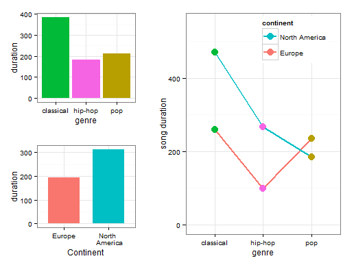
The inclusion of multiple variables in an ANOVA allows you to examine another interesting phenomenon: the interaction effect. If there is an interaction between two factor variables, it means that the effect of either factor on the response variable is not the same at each category of the other factor. The easiest way to understand an interaction effect at play is to visualize the effect.

The visualization above contains 3 parts. The left top visualization contains the main effect of genre on song duration. As you can see, the pop and hip-hop genres are fairly similar to each other but a classical song has a much longer duration on average. This is where the significance of the genre variable comes from. The left bottom visualization contains the main effect of continent. As you can see, North American songs have on average a longer duration than European songs. However, if you look at the right most plot, you see that this pattern holds for North American and European classical and hip-hop songs but not for pop songs. European pop songs have a higher song duration than American pop songs. This is exactly what is meant with the statement that the effect of either factor on the response variable is not the same at each category of the other factor.
In MatLab, you include an an interaction term in your model by adding the 'interaction' argument into the anovan function, like this: |[p,tbl,stats] = anovan(y, {g1,g2,g3}, 'model', 'interaction'). In multcompare(), to get an overview of which group of which level differs from others, and how, add the following arguments to the function call: multcompare(stats,'Dimension',[1 2],'alpha',0.05)
- For the current exercise, all our data is available in the dataframe `songdata2`. Conduct a two-way ANOVA using the `anovan()` function with an interaction between the variables genre and continent and request [p,tbl, stats] as outputs.
- Call multcompare on `stats', use the default post hoc test and print the output to the console.
In the last exercise, we created a model with two main effects and 1 interaction effect. In this exercise we will interpret the interaction effect. Usually you would follow up an interaction effect to get more information on how to interpret your interaction effect. This is however beyond the scope of this course. To see once again what the interaction looks like, see the graph below:

Choose the best interpretation of the interaction effect as displayed in the graph above
- The effect of genre on song duration becomes insignificant once the continent variable is included
- The effect of genre is similar for European songs as for North American songs
- The effect of genre on song duration differs between European and North American songs