Level(3) Lambda UDPmon Large with STS Tuning
Description
UDPmon
In this document UDP experiments are described that were performed with a
modified version of the UDPmon
package written by R.E. Hughes-Jones in the sense that from
5000 packets the sequence number and the arrival time in microsec. are
specified. All packets were send with zero sec. wait time between two
successive packets. The experiments were executed at the
Level(3) Lambda before acceptance by
SURFnet. All tests were performed after the
hosts upgrade of the SARA cluster to
515 Mbyte memory and Linux V.2.4.16-web100.
Network bottleneck memory estimation
UDPmon tests, that are
executed by the workstations with a speed that exceeds the limits the network
equipment or line can handle, in general show the following two characteristic
phases:
-
In the first part of the test the memory in the network is able to buffer
the packets that can be handled at line speed, so nothing will be dropped.
-
At the moment the memory has been completely filled, the equipment is unable
to keep up with line speed and handle all incoming packets, so typically
packet drop will occur in this phase.
This characteristic behaviour can be used to estimate the amount of memory that
has been installed in the equipment which forms the bottleneck in the current
path. Calculate the rate of packets dropped in
phase 2 of the
UDPmon test, given by
with:
|
rdrop 2
|
|
: |
|
The drop rate calculated in
phase 2.
|
|
Ndrop 2
|
|
: |
|
The # packets dropped in
phase 2.
|
|
Nall 2
|
|
: |
|
The total # packets send during
phase 2.
|
Under the assumption that the bandwidth in the
phases 1
and 2 are the same,
can be used to calculate the available memory in the network equipment that
forms the bottleneck. In that case the value of the drop rate for
phase 2 can also be used for the
first phase. at the end of that phase the
network equipment memory is just filled and should be:
with:
|
Mnet
|
|
: |
|
The amount of memory in the network equipment forming the
bottleneck.
|
|
rdrop 2
|
|
: |
|
The drop rate calculated in
phase 2.
|
|
Nall 1
|
|
: |
|
The total # packets send and received during
phase 1.
|
|
Spacket
|
|
: |
|
The packet size.
|
|
SUDP
|
|
: |
|
The UDP overhead. It is assumed to be 64 byte.
|
To obtain reliable results the packet drop rate in
phase 2 can be set to more reliable values
my limiting the provisioned bandwidth. Of course this also implies that the
total # packages received without loss in
phase 1 is lowering, so for some value
of the provisioned bandwidth there is an optimum to determine the involved
memory
with .
The provisioned bandwidth can be varied by setting the appropriate
STS (Synchronous Transport Signal) level at the Cisco ONS. The
levels, displayed in
,
can be selected.
STS
Level |
Bandwidth
[Mbit/s] |
| 1 |
55 |
| 3C |
155 |
| 6C |
311 |
| 9C |
466 |
| 12C |
622 |
| 24C |
1250 |
| . |
|
The used
STS levels with the corresponding provisioned
bandwidths. |
Test setup
For these tests the topology described in
has been used. In this figure only the part of the setup essential for these
tests are shown. There follows that the route via the Gigabit interfaces between
gwgsara3 and gwgsara5 is formed by the path
Amsterdam - Chicago - Amsterdam, where both
Cisco ONS's are the only involved network equipment. The whole path
between the two hosts forms one VLAN. At the points marked
with "C" appropriate
SNMP counters are available to check for packets lost.
+--------+   C +-+        +-+
|gwgsara3|-----|O|        |O| C
+--------+     | |- .... -| |--+
               |N|        |N|  | hardware loop
+--------+     | |- .... -| |--+
|gwgsara5|-----|S|        |S| C
+--------+   C +-+        +-+

      SARA                Chicago
|
| . |
|
The topology of the test setup used. Only the
components required for these tests are shown. At the
positions marked with "C"
the appropriate SNMP counters are read to check for
losses. |
Tests between gwgsara3 and gwgsara5
With the modified version of the
UDPmon tool tests between the
hosts gwgsara3 and gwgsara5 has been performed while the STS
levels are varied in correspondence with
.
Before and after each test the appropriate SNMP counters (see
)
have been read to check for packets lost.
Time-Sequence
Results
To demonstrate the two phase behaviour of the
UDPmon tool, described in the
"Description" section, the relative
receiving time of the packets after the first packet has been displayed as a
function of the packet sequence number. The results are displayed for STS-12C
(622 Mbit/s) because at that speed the effects are clear visible. STS-12C
is also a common used standard. In the
the relative receiving time has been plotted as a function of the packet
sequence number using the packet sizes 500 byte, 1000 byte,
1200 byte, and 1460 byte for the stream gwgsara3 =>
gwgsara5. In
these data are presented for the reverse stream. Lost packets are marked in
these figures with zero relative receiving times.
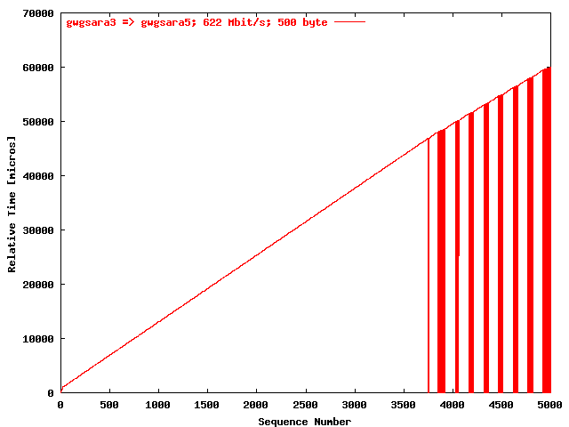
| .I. |
|
The relative receiving time as function of the packet
sequence number for the UDP stream
gwgsara3 => gwgsara5. The
packet size was 500 byte. |
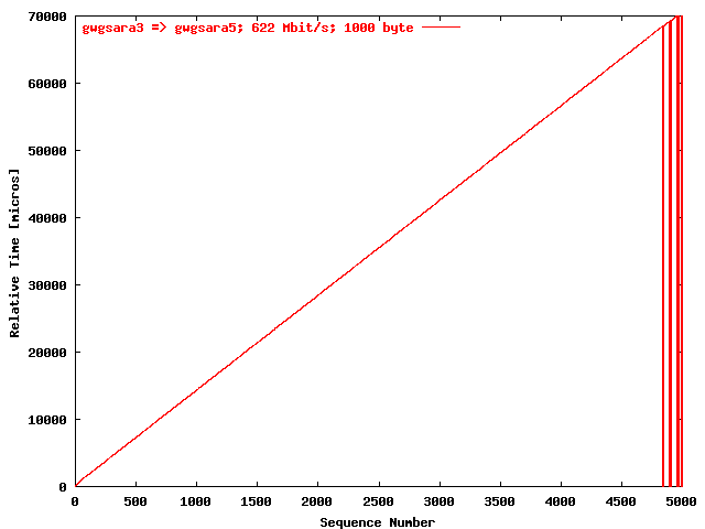
| .II. |
|
The relative receiving time as function of the packet
sequence number for the UDP stream
gwgsara3 => gwgsara5. The
packet size was 1000 byte. |
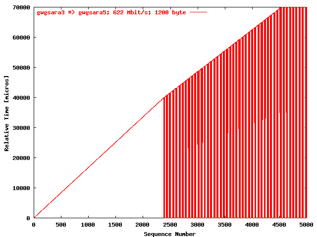
| .III. |
|
The relative receiving time as function of the packet
sequence number for the UDP stream
gwgsara3 => gwgsara5. The
packet size was 1200 byte. |
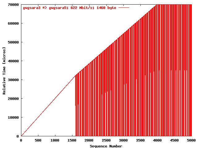
| .IV. |
|
The relative receiving time as function of the packet
sequence number for the UDP stream
gwgsara3 => gwgsara5. The
packet size was 1460 byte. |
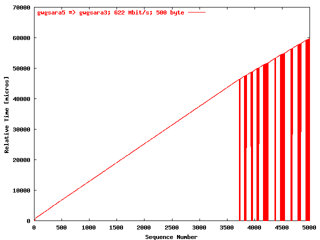
| .I. |
|
The relative receiving time as function of the packet
sequence number for the UDP stream
gwgsara5 => gwgsara3. The
packet size was 500 byte. |
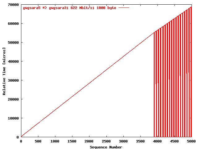
| .II. |
|
The relative receiving time as function of the packet
sequence number for the UDP stream
gwgsara5 => gwgsara3. The
packet size was 1000 byte. |
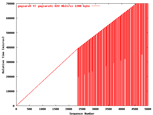
| .III. |
|
The relative receiving time as function of the packet
sequence number for the UDP stream
gwgsara5 => gwgsara3. The
packet size was 1200 byte. |

| .IV. |
|
The relative receiving time as function of the packet
sequence number for the UDP stream
gwgsara5 => gwgsara3. The
packet size was 1460 byte. |
Conclusions
From the
the following conclusions can be drawn:
-
The partitioning in a phase 1,
where no packets are dropped because the network memory is still being
filled, and a phase 2, where packets
are dropped, could be found in all figures.
-
With increasing packet size, the # packets from
phase 1, that could be received
without lost, is shifting to the left, as could be expected. The only
exception is for a packet size of 500 byte. That is probably due to
host effects. With the smaller packet sizes the amount of interrupt levels
that could be handled form a bottleneck.
-
No relevant differences between the two stream directions could be found,
although gwgsara5 has a slightly better performance than
gwgsara3: 1000 MHz compared with 860 MHz.
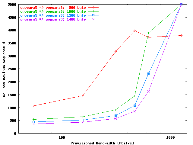
Phase 1 Maximum Sequence Number
Results
To show the increasing # packets from
phase 1 by an increasing provisioned
bandwidth (increasing STS levels), the maximum sequence number without loss has
been plotted as function of the provisioned bandwidth, determined by the
adjusted STS level. Packet sizes of 500, 1000, 1200, and 1460 byte are
used from which the results are represented by corresponding plot traces. In
these data are specified for the stream gwgsara3 =>
gwgsara5 and in
for the reverse direction.
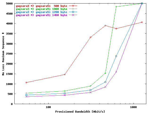
| . |
|
The maximum sequence # that could be send without
loss (defining the length of the
phase 1
region) as function of the provisioned bandwidth for the
stream gwgsara3 => gwgsara5.
The data for the used packet sizes are represented by
corresponding plot traces. |
| . |
|
The maximum sequence # that could be send without
loss (defining the length of the
phase 1
region) as function of the provisioned bandwidth for the
stream gwgsara5 => gwgsara5.
The data for the used packet sizes are represented by
corresponding plot traces. |
Conclusions
From the
the following could be concluded.
-
For the smallest provisioned bandwidth (55 and 155 Mbit/s) the
size of the phase 1 is
unchanged for all packet sizes except 500 byte, indicating that in this
region the transfer rate is completely limited by the value of the
provisioned bandwidth.
-
For the bandwidths above 155 Mbit/s the
phase 1 region is indeed
increasing by increasing provisioned bandwidth.
-
Only for a packet size of 500 byte the growth stops at a bandwidth of
466 Mbit/s. This is probably due to host limitations.
-
No significant differences between both stream direction could be found.
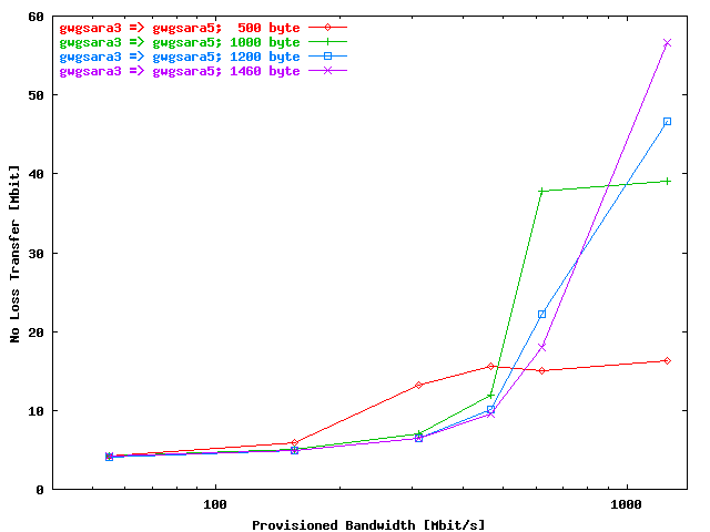
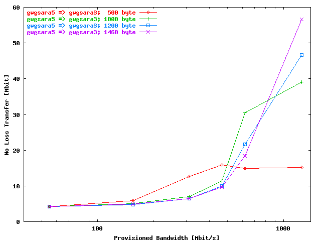
Data Transfer during Phase 1
Results
From the packet size plot traces in the
,
shown in the previous section, the
impression may arise that the in
phase 1 transferred data bulk also
contains characteristic behaviour. Therefore, the
phase 1 transferred data has been
plotted here as a function of the provisioned bandwidth. Also in these plots the
used packet sizes are represented by separate plot traces. In
these data are presented for the stream gwgsara3 =>
gwgsara5 and in
for the reverse direction. The UDP overhead of 64 byte has been
included in the calculation of the amount transferred data.
| . |
|
During
phase 1,
without packet loss, transferred data bulk as function
of the provisioned bandwidth in the direction
gwgsara3 => gwgsara5. The used
packet sizes are represented by separate plot
traces. |
| . |
|
During
phase 1,
without packet loss, transferred data bulk as function
of the provisioned bandwidth in the direction
gwgsara5 => gwgsara3. The used
packet sizes are represented by separate plot
traces. |
Conclusions
From the
the following can be concluded:
-
For the smaller provisioned bandwidths (55 and 155 Mbit/s) the
transferred data are the same for all packet sizes. This implies that the
transfer rate is completely limited by the provisioned bandwidth, as could
be expected.
-
For the intermediate provisioned bandwidths (311 Mbit/s,
466 Mbit/s, and for packet sizes > 500 byte also for
622 Mbit/s) it is possible to transport more data with smaller packet
sizes.
For smaller packets sizes this behaviour becomes more
significant for smaller provisioned bandwidths. Obviously is the chance at a
packet drop for smaller packet sizes considerably smaller than for larger
packet sizes, resulting in a considerable larger
phase 1 drop-less area. See also
the
.
However, a good explanation for these differences in drop-less areas we do
not have.
-
For the larger provisioned bandwidth (622, and 1250 Mbit/s) the
transferred data for the packet size of 500 is limited by host effects
as could also be seen from the
.
-
No significant differences could be observed between both stream directions.
Number Packets Lost
Results
In this section the # packets lost during
phase 2 has been plotted as a function of
the provisioned bandwidth. The data for the used packet sizes are presented by
corresponding plot traces.
displays the # lost packets for the stream gwgsara3 =>
gwgsara5 and
for the reverse direction.
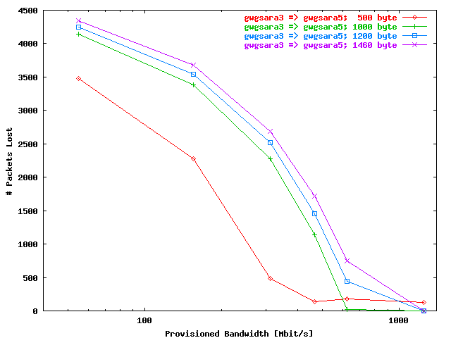
| . |
|
The # packets lost as a function of the
provisioned bandwidth for the stream
gwgsara3 => gwgsara5. The used
packet sizes are represented by separate plot
traces. |
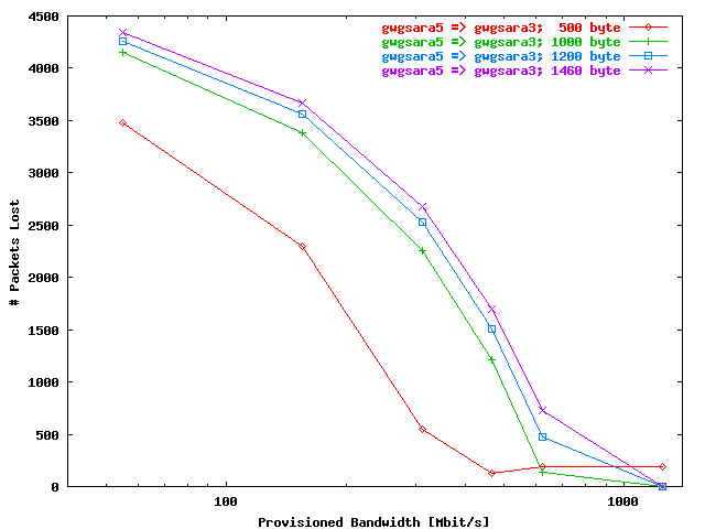
| . |
|
The # packets lost as a function of the
provisioned bandwidth for the stream
gwgsara5 => gwgsara3. The used
packet sizes are represented by separate plot
traces. |
Conclusions
Unsurprisingly about the same characteristics can be seen as in the previous
"Phase 1 Maximum Sequence Number" and
"Data Transfer during Phase 1" sections, because the data
presented here are related with those data. From the
there follows:
-
The # packets lost per provisioned bandwidth is increasing with
increasing packet size. The provisioned bandwidth here is limiting the
UDP throughput.
-
For the packet size of 500 byte host dependent packet losses are
occurring for provisioned bandwidths >= 622 Mbit/s.
-
No significant differences could be observed between both stream
directions.
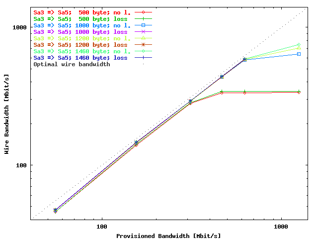
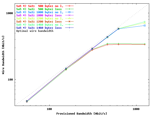
Bandwidth in Regions with & without Packets Loss
Results
To check the assumptions that the bandwidth in the regions with and without
packets lost (phases 1
and 2) are the same, the wire bandwidths
(also with 64 byte UDP overhead included ) have been plotted as
function of the provisioned bandwidth. Note that the bandwidths are only
calculated in both regions when there are 200 or more non-zero relative time
stamps available. In
the wire bandwidths are presented for the direction gwgsara3 =>
gwgsara5 and in
for the reverse direction. The data for the used packet sizes are given in the
corresponding plot traces. The optimal situation where the wire bandwidth is
equal to the provisioned bandwidth has been marked with a dotted line.
| . |
|
The wire bandwidth in the regions without packet loss
(phase 1,
marked with "no l."), and with
packet loss
(phase 2, marked
with "loss") as a function of the
provisioned bandwidth for the direction
gwgsara3 => gwgsara5. The used
packet sizes are presented with separate plot traces.
The optimal situation where the wire bandwidth is equal
to the provisioned bandwidth has been marked with a
dotted line. |
| . |
|
The wire bandwidth in the regions without packet loss
(phase 1,
marked with "no l."), and with
packet loss
(phase 2, marked
with "loss") as a function of the
provisioned bandwidth for the direction
gwgsara5 => gwgsara3. The used
packet sizes are presented with separate plot traces.
The optimal situation where the wire bandwidth is equal
to the provisioned bandwidth has been marked with a
dotted line. |
Conclusions
From the
the following conclusions can be drawn:
-
No significant differences between the
phase 1) and
phase 2 regions could be observed, so
the assumption leading to
seems to be correct. Note that for a provisioned bandwidth of
1250 Mbit/s there are for packet sizes > 500 byte too few
data available to calculate reliable the
phase 2 bandwidth values.
-
The achieved wire bandwidth values are close to the optimal values limited
by the provisioned bandwidth, until the wire bandwidth is limited by host
effects for
-
500 byte packet size and provisioned bandwidths of
>= 466 Mbit/s.
-
>= 1000 packet sizes and a provisioned bandwidth of
1250 Mbit/s.
-
No significant differences could be observed between both stream
directions.
Network Bottleneck Memory
Results
As in the previous section has been shown it is allowed
to use
to calculate the memory of the network bottleneck using the appropriate
# packets received and/or lost in the
phases 1
and 2. In
the network memory has been plotted as function of the provisioned bandwidth for
the direction gwgsara3 => gwgsara5 and in
for the reverse direction. The estimation for the network bottleneck memory is
only executed when 100 or more packets are lost.
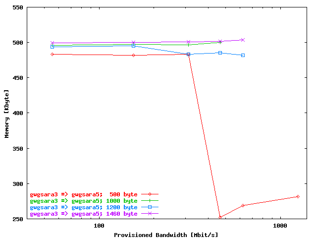
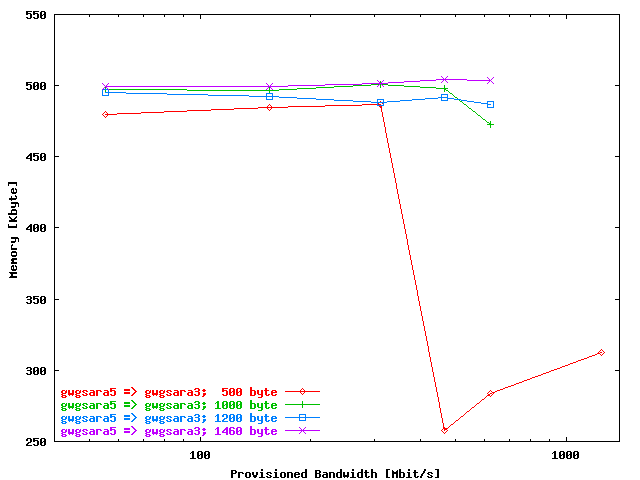
| . |
|
The network bottleneck memory as a function of the
provisioned bandwidth for the direction
gwgsara3 => gwgsara5. The used
packet sizes are represented with corresponding plot
traces. |
| . |
|
The network bottleneck memory as a function of the
provisioned bandwidth for the direction
gwgsara5 => gwgsara3. The used
packet sizes are represented with corresponding plot
traces. |
Conclusions
The following conclusions can be drawn from the
:
-
Reasonable consistent results can be obtained for provisioned bandwidths
<= 622 Mbit/s. For a provisioned bandwidth of 1250 Mbit/s,
there are insufficient, or none, packets lost.
-
For a packet size of 500 Mbit/s no reliable memory estimates could be
obtained for provisioned bandwidth >= 466 Mbit/s. As reported
before, this has been caused by packets lost due to host effects.
-
The estimated value for the memory of about 500 Kbyte does not seems to
be unrealistic.
-
No significant differences could be observed between both stream directions.
SNMP Counters
Results
In this section the results are presented from the SNMP In & Out Octet
counter evaluations that were executed at the Cisco ONS's at the
interfaces marked
with "C" at the setup scheme given in
.
According to this scheme
lists the Octet In and Octet Out counters that could be
compared with each other to check for packet loss.
|
Step
|
Octet In
|
Octet Out
|
|
1.
|
Amsterdam host interface
|
Chicago hardware loop
|
|
2.
|
Chicago hardware loop
|
Chicago hardware loop
|
|
3.
|
Chicago hardware loop
|
Amsterdam host interface
|
| . |
|
Octet In counters that are compared with the
corresponding Octet Out counters to check for
packet loss. |
The corresponding Octet In & Out counters were read
before and after each UDPmon
performance test. A comparison of the appropriate counter differences, after and
before each test, gives the # Octets lost during that test which can also
be roughly expressed in the # packets lost by dividing it by the sum of the
packet size and the UDP overhead (64 byte).
Probably it is not very surprising that only octet loss has been found for those
counters which are compared in step 1
from
,
because by limiting the provisioned bandwidth, the Amsterdam Cisco ONS
forms the bottleneck in the setup given by
.
These octet and packet losses are presented by the following plots.
displays the # Octets lost for the stream gwgsara3 =>
gwgsara5 and
for the reverse direction. The Octets lost converted to the # packets lost
for these streams can be found in the
,
respectively. To be able to compare easily the SNMP results with the
# packets lost, obtained with
UDPmon, also these results
have been add to the last two figures.
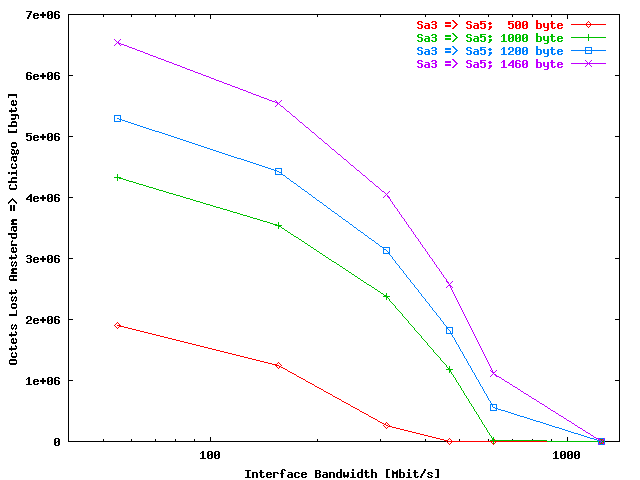
| . |
|
The Octets lost from the Amsterdam host to the Chicago
hardware loop as a function of the provisioned bandwidth
for the direction gwgsara3 =>
gwgsara5. The used packet sizes are presented
with separate plot traces. |
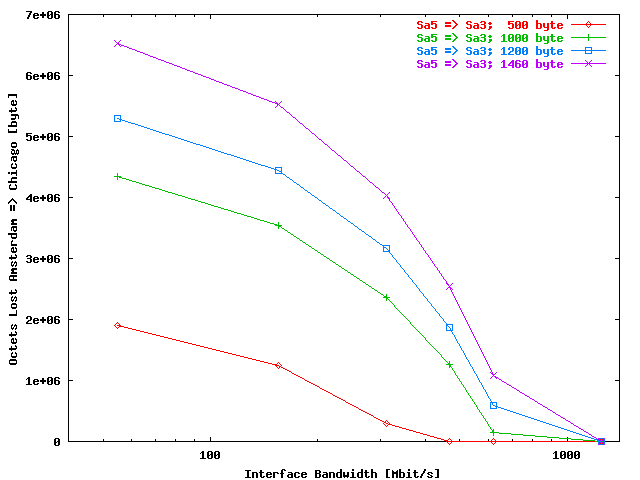
| . |
|
The Octets lost from the Amsterdam host to the Chicago
hardware loop as a function of the provisioned bandwidth
for the direction gwgsara5 =>
gwgsara3. The used packet sizes are presented
with separate plot traces. |
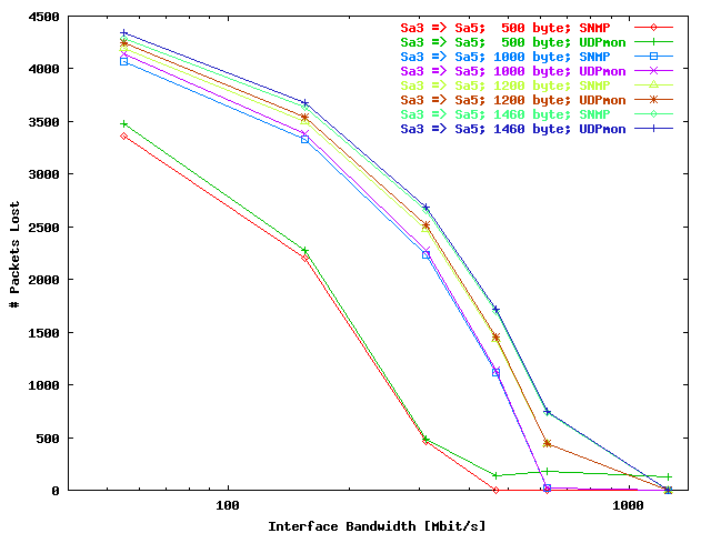
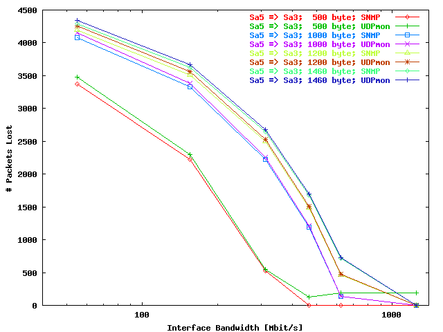
| . |
|
The # packets lost as a function of the
provisioned bandwidth for the direction
gwgsara3 => gwgsara5. The used
packet sizes are presented with separate plot traces.
The traces marked with "SNMP" are
referring to the SNMP # packets lost from the
Amsterdam host to the Chicago hardware loop, while the
traces marked with "UDPmon" are
pointing to the UDPmon results, also previously
presented in . |
| . |
|
The # packets lost as a function of the
provisioned bandwidth for the direction
gwgsara5 => gwgsara3. The used
packet sizes are presented with separate plot traces.
The traces marked with "SNMP" are
referring to the SNMP # packets lost from the
Amsterdam host to the Chicago hardware loop, while the
traces marked with "UDPmon" are
pointing to the UDPmon results, also previously
presented in . |
Conclusions
From the
the following conclusions can be given:
-
There is a good agreement between the packets lost, calculated from the
Octet counters, and the results obtained with
UDPmon, especially for
provisioned bandwidths >= 311 Mbit/s.
-
The SNMP results also form an indication that the packets lost encountered
at a packet size of 500 byte for provisioned bandwidths
>= 466 Mbit/s are indeed caused by host effects, because the
Octet counters did not show any loss for these provisioned bandwidths.
-
No significant differences could be observed between both stream directions.
General Conclusions
From the tests where the provisioned bandwidth has been limited by tuning the
STS level at the Cisco ONS and sending UDP packets with
the UDPmon tool, the following
conclusions can be drawn:
-
With
a reasonable estimation of the memory from the network bottleneck seems to
be possible. However, the assumption, that the bandwidth is the same in the
regions during the tests before and after the memory has been filled (the so
called phases 1
and 2), has to be verified. In our
case this assumption seemed to be valid.
-
Limiting the provisioned bandwidth was in our situation required to obtain a
condition where the extensions of both phases are large enough to make the
calculation
of
sufficient reliable. Without limiting the provisioned bandwidth too few
packets were lost.
-
The calculation of the memory
using
is consistent in a relatively large range of provisioned bandwidths and used
packet sizes.
-
The monitoring of SNMP counters at the network equipment before and after
the tests may help to eliminate possible host dependent effects.
-
Not much influence could be noticed from the better performance of host
gwgsara5 (1000 MHz) compared with gwgsara3
(860 MHz), but these differences are not very large either.
^ All Level(3) Lambda UDPmon Large Results |
Teleglobe Lambda UDPmon Large Results