 |
Generalizations of BST (bintree) to QST (quadtree) and OST (octtree).
The BST has been based on a domain of keyvalues. The key of the root,
say k, divides this domain into two parts:
•	the lhs subtree contains keys smaller than k
•	the rhs subtree contains keys larger  than k.

The idea can be immediately generalized to 2-dimensional keys say [x,y].
Then the key [k',k"] of the root element divides this domain into
4 parts (x smaller or larger than k', and also y smaller or larger than k".
These 4 parts are called quadrants.
Each treenode now has 4 subtrees, one for each of the quadrants, and
the tree is called a QST(quad search tree).
Similarly, 3-dimensional keys [k,k',k"] are from a domain of search of
the form [x,y,z] and a specific key [k,k',k"] divides this domain into
8 octants.
Each treenode now has 8 subtrees, one for each of the octants, and
the tree is called an OST(oct search tree).

Modifying the interface and the implementation of BST to QST and OST is
not difficult although it takes some time from setup to endoftesting.
|
API

|


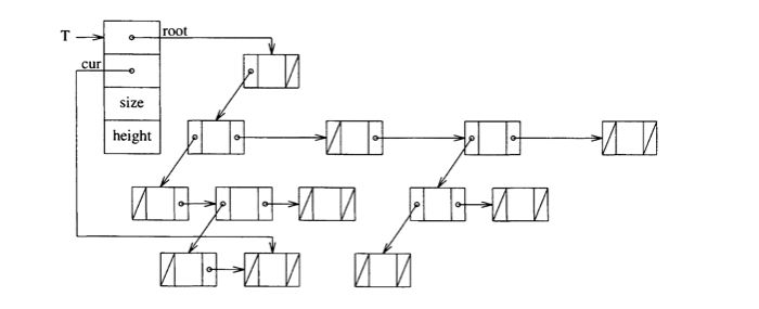 NB: The
 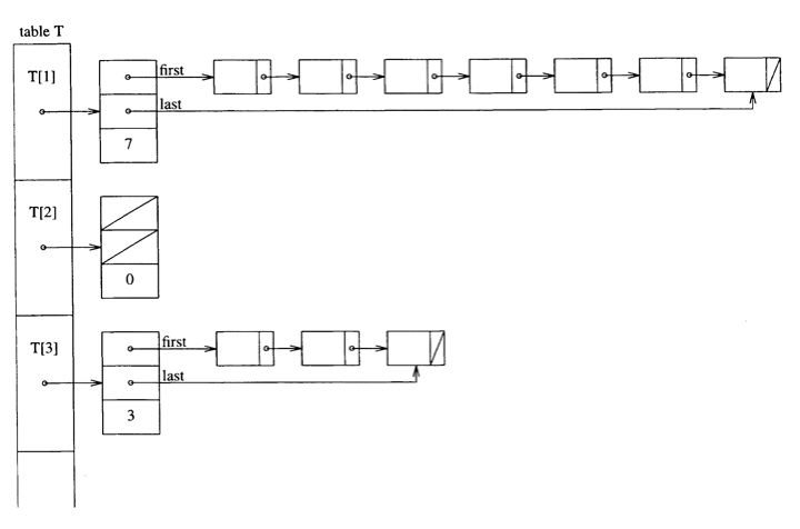 The declaration can be written from this picture.
 and again, the declaration can be written from this picture.
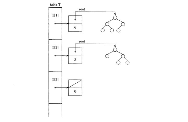
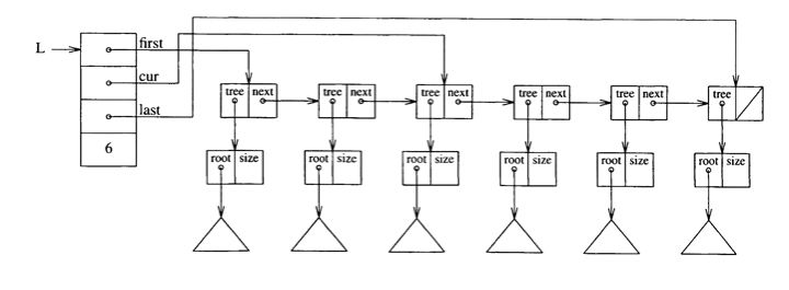 The declaration of the trees can be taken from the previous section and
the list is defined on the next sheet:
The declaration of the trees can be taken from the previous section and
the list is defined on the next sheet: