Lab Exercise Probability I¶

Throwing a fair dice¶

1. What is the probability space \(U\) if we throw once with a dice.
2. We throw the same dice twice. What is the probability space for this experiment?
3. What is the probability to throw a six twice?
4. What is the probability to get 9 points in total in two throws?

Venn Diagram¶

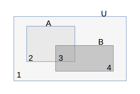
Fig. 1 Venn Diagram for 2 events \(A\) and \(B\) in universe \(U\). Also indicated are the 4 elementary regions in the Venn diagram.

Consider the Venn diagram for events \(A\) and \(B\) in universe \(U\). It is given that:

1. The elementary region with label 3 corresponds with the event \(A\cap B\). Give the events (in terms of \(A\), \(B\) and \(U\)) of the other three elementary regions.
2. Calculate the probabilities of the four events defined in the previous question.

Axioms and Theorems of Probability¶

1. Prove that \(\P(A\cup B) = \P(A) + \P(B) - \P(A\cap B)\) using the axioms of probability. Start with a ‘graphical proof’ based on a Venn diagram. Can you also give a formal algebraic proof (i.e. manipulating equations).

2. Also prove \(\P(A) = \P(A\cap B) + \P(A\cap \neg B)\). Again give a graphical proof as well as a algebraic proof.

3. Let \(B_i\) for \(i=1,\ldots,n\) form a partition of \(U\), prove that:

   \[\P(A) = \sum_{i=1}^{n} P(A\cap B_i)\]

Conditional Probability and Bayes Rule¶

1. We have seen that \(\P(A) + \P(\neg A) = 1\). What about \(\P(A\given B) + \P(\neg A\given B)\) ?

2. We have seen that \(\P(A) + \P(\neg A) = 1\). What about \(\P(A\given B) + \P(\neg A\given C)\) ?

3. We have seen that \(\P(A) + \P(\neg A) = 1\). What about \(\P(A\given B) + \P(A\given \neg B)\) ?

4. Prove Bayes rule:

   \[\P(A\given B) = \frac{\P(A)}{\P(B)}\,\P(B\given A)\]

Chain Rule¶

1. Prove the chain rule:

   \[\P(A_1 A_2 \cdots A_n) = \P(A_1 \given A_2 \cdots A_n)\,\P(A_2\given A_3 \cdots A_n) \cdots \P(A_{n-1}\given A_n) \, P(A_n)\]

   starting from the definition of the conditional probability. Note that we use \(A B\) to denote the event \(A\cap B\).

2. The above chain rule is not unique. Give a second form for the chain rule. How many different forms can you come up with?

Marbles and Vases¶

Consider the following experiment: we have three vases labeled 1, 2 and 3. In every vase there are a number of red and white marbles given in the following table:

Vase	#Red	#White
1	1	5
2	1	2
3	1	1

First we select one of the vases. There is no preference for one of the vases. Then from the choses vase we pick one marble.

The random experiment is described with two random variables: \(V\) (vase) with posible outcomes 1,2 and 3, and \(C\) for the color of the marble.

1. Draw the probability tree for this random experiment and calculate \(\P(C=\text{'white'})\) .

2. Without a doubt you have multiplied probabilities in the calculations in the tree. Which rule from probability theory have you (implicitly) applied many times when making the tree.

3. The tree you have just made start by selecting a vase, and then picking a marble. This is of course according to the causality of the random experiment.

   Probability theory is however not about causality. We can equally well make a tree where we first split according to the color of the marble and then according to the vase and still come up with the same probabilities for all possible combinations of vase and color.

   Draw this tree as well and calculate all probabilities.

Naive Bayesian Classifier¶

In this exercise you have to implement the Naive Bayesian Classifier in Python/Numpy. The goal is to classify a person as either female ( \(X=1\) ) or male ( \(X=0\) ) based upon the 3 features: length (r.v. \(L\) ), weight (r.v. \(W\) ) and shoe size (r.v. \(S\) ). These 3 features are assumed to be class conditionally normally distributed.

We have a comma separated file of examples from the 2014 class. For each student the values of \(X\), \(L\), \(W\) and \(S\) are tabulated in the file. Note there are many ways to read the data in a csv file in Python. Do not write this yourself. The data can be downloaded here.

Your tasks for this exercise are:

1. Write a section in which you start with the Bayes Classifier for this problem using the symbols ( \(X,L,W\) and \(S\) ) that are introduced in this exercise and end with the formula for the naive Bayesian classifier.
2. Estimate the parameters of the six normal distributions that are needed for classification. Give all parameters in a table in your report. And plot the conditional probability density functions. For each random variable plot the pdf for both female and male in one plot.
3. Test your classifier on the same data that is used to learn. Yes, this is a big no-no in machine learning! For this first example of a machine learning algorithm we make an exception. Present the results in a confusion matrix (see Wikipedia for the definition).

Some Random Programming¶

(This exercise is not needed in your portfolio, it is just for fun).

Fig. 2 A Galton board of 7 layers.

In this exercise we will simulate a Galton board. The basic random experiment in a Galton board is a small spherical ball vertically falling and hitting a small pin. The ball is restricted to move in two dimensional plane and thus is forced to go to the left or right of the pin. Probability of going left is \(\P(L)\) and that of going right is \(\P(R)\).

Then just below the first pin when the ball falls to the left, is another pin. Then the ball is again forced to go left or right. The same is done for the ball hitting the top most pin and goes right.

Note that a ball first going left and then right ends up in the same position as ball first going right and then going left.

Along the same line of reasoning we can add more layers of pins to obtain a Galton board of \(n\) layers. The path a marble takes when falling down and going left or right \(n\) times is characterized as a string of length \(n\) of only L’s and R’s.

The position where the ball ends up is given by the number of ‘R’s in the string (when we number the positions from \(0\) to \(n\) goint from left to right).

For this exercise you should write a function galtonSimulate(n, N) where n is the number of layers in the Galton board and \(N\) is the total number of balls that are dropped. The function should return a numpy array \(A\) of shape \((n+1,)\) where \(A[i]\) is the number of balls that end up in bin \(i\), for \(i\) is \(0\) to \(n\) .

The random number generator that you are allowed to use is numpy.random.randint. This generator can be used to draw numbers 0 and 1 each with probability 0.5.

As allways in numpy you should be careful to avoid explicit loops in Python.

Visualize \(A[i]\) with a bar plot for \(n=10\) and \(N = 100000\) . Also scale the values of \(A[i]\) to make it into an estimate of the probability \(\P(i)\) that a ball ends up in bin \(i\) .

For bonus points: can you calculate the probability that a ball will end up in bin \(i\) ?