Normal Distributed Random Vectors¶

Definition¶

The multivariate normal distribution of an n-dimensional random vector is defined as:

\[f_{\v X}(\v x) = \frac{1}{(2\pi)^{n/2} |\v \Sigma|^{1/2}} \exp\left( -\tfrac{1}{2}(\v x - \v \mu)\T \v \Sigma^{-1} (\v x-\v\mu) \right)\]

We can also define the multivariate normal distribution with the statement that a random vector \(\v X\) has a normal distribution in case every linear combination of its components is normally distributed, i.e. for any scalar vector \(a\) the univariate (or scalar) random variable \(Y = \v a\T\v X\) is normally distributed.

The normal distribution is completely characterized with its expectation and (co)variance:

\[\begin{split}\E(\v X) = \v\mu \\ \Cov(\v X) = \v\Sigma\end{split}\]

As an example consider the two dimensional normal distribution with

\[\begin{split}\v \mu = \matvec{c}{8\\5}\\ \Sigma = \matvec{cc}{1 & 1 \\ 1 & 2}\end{split}\]

Plotting 500 samples from this distribution gives an impression of the probability density function. Where a lot of samples cluster on the plane the density will be high and it will be lower where less samples are.

In [1]: from pylab import *

In [2]: mu = array([8,5])

In [3]: S = array([[1,1],[1,2]])

In [4]: w,v=eigh(S)

In [5]: T = dot(v,diag(sqrt(w)))

In [6]: x = randn(500,2)

In [7]: y = dot(T,x.T).T + mu

In [8]: plot(y[:,0],y[:,1],'.g')

In [9]: axis('equal')

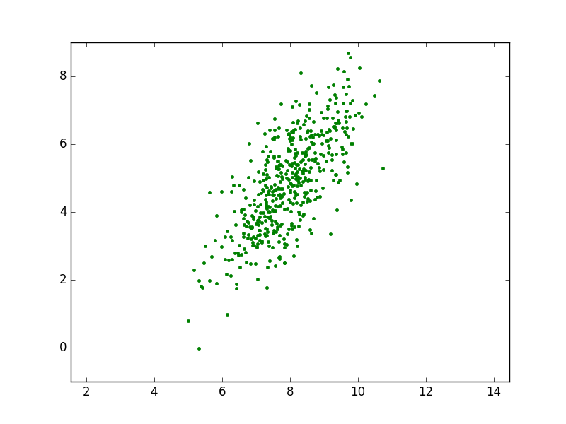
From the scatter plot we can infer that the mean value of the samples is indeed somewhere near the point \((8,5)\). The distribution is clearly elongated in an (almost) diagonal direction. In the next section we will show how to relate the covariance matrix with the ‘shape’ of the scatterplot.

For this distribution we can of course make a nice plot of the probability density function itself:

In [10]: mu = array([8,5])

In [11]: S = array([[1,1],[1,2]])

In [12]: from mpl_toolkits.mplot3d.axes3d import Axes3D

In [13]: fig = plt.figure()

In [14]: ax = fig.add_subplot(1, 1, 1, projection='3d')

In [15]: X = np.arange(4, 12, 0.1)

In [16]: Y = np.arange(0, 10, 0.1)

In [17]: X, Y = np.meshgrid(X, Y)

In [18]: X = X-mu[0]; Y = Y - mu[1];

In [19]: Si = inv(S)

In [20]: f = 1.0/(2*pi*sqrt(det(S)))*exp(-(Si[0,0]*X**2 + 2*Si[0,1]*X*Y + Si[1,1]*Y**2))

In [21]: surf = ax.plot_surface(X, Y, f, rstride=1, cstride=1,
   ....:           cmap=cm.summer, linewidth=0, antialiased=False)
   ....:

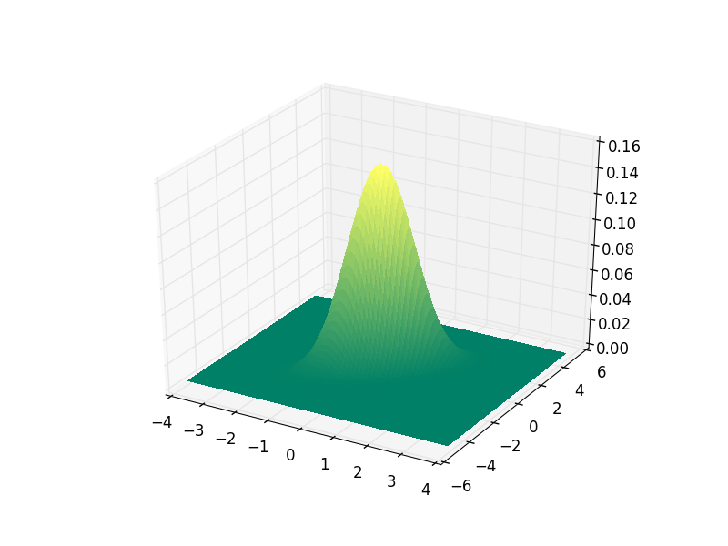
If you run this code and plot the pdf in a separate window (not in a notebook) you can interactively scale and rotate the plot to make the 3D geometry better visible.

Geometry¶

In order to get a feeling for the ‘shape’ of the distribution we look at the isolines of the probability density function \(f_{\v X}(\v x)=\text{constant}\). Assume that \(\v \mu = \v 0\), i.e. the distribution is centered at the origin. Then

\[\v x\T \Sigma\inv \v x = \text{constant}\]

Since the covariance matrix is symmetric (and thus its inverse is too) we recognize a quadratic form: \(\v x\T Q \v x\) with a symmetric matrix \(Q=\Sigma\inv\).

Remember from linear algebra class that a quadratic form can always be diagonalized, i.e. we can find an orthogonal basis in which the covariance matrix is diagonal.

Let \(\v Y = A \v X\). then we have found that:

\[\Cov(\v Y) = \Cov(A\v X) = A\Cov(\v X) A\T\]