5.4.1. Physical Modelling of Dynamic Systems

In control theory the Laplace transform plays an important role. Using the Laplace transform the constant coefficient linear differential equations that model physical systems can be transformed into algebraic equations.

In this section we give two examples of physical systems (a thermodynamical first order system and a mechanical second order system).

For a control engineer the differential equations are the starting point. Modelling the physical systems is most often the task of other specialists.

In this course we don’t expect our students to be able to model physical (or other systems) with differential equations.

5.4.1.1. Warming Up

Consider a block of aluminium kept in the fridge at zero degrees for a long time so the block is at that temperature as well. Now at time \(t=0\) we get that block of alumimium out of the fridge and bring it to a room with a constant temperature of twenty degrees.

After a while the block of aluminium will be 20 degrees as well. But how long does that take? And in what way will the temperature change from zero to twenty degrees Celcius.

The heat transfer from the aluminium block to its surroundings is proportional to the difference between the temperature of the block and the temperature of its surroundings. In control theory the temperature is often denoted with the symbol \(q\) to distinguish it from time. The heat flow is:

\[F = h A_s (q_b(t) - q_s(t))\]

where \(q_b\) is the temperature of the block and \(q_s\) is the temperature of its surroundings.

If heat is transferred from the block to its surroundings its temperature will drop according to:

\[\rho c_p V \frac{d q_b(t)}{d t} = -F\]

where \(\rho\) is the density of the block, \(c_p\) is the specific heat and \(V\) is the volume. Combining the two equations we get:

\[\rho c_p V \frac{d q_b(t)}{d t} = - h A_s (q_b(t) - q_s(t))\]

Rearranging terms leads to:

\[\rho c_p V \frac{d q_o(t)}{d t} + h A_s q_b(t) = h A_s q_s(t)\]

Using

\[\tau = \frac{\rho c_p V}{h A_s}\]

we get:

\[\tau \frac{d q_b(t)}{d t} + q_b(t) = q_s(t)\]

Taking the Laplace transform on both sides we get:

\[\tau s Q_b(s) + Q_b(s) = Q_s(s)\]

or

\[H(s) = \frac{Q_b(s)}{Q_s(s)} = \frac{1}{\tau s + 1}\]

This is the transfer function of a classical first order system. In a later section we will look at its impulse, step and frequency response more formally. There it will be shown that the step response for this thermal system looks like (where we have assumed the time constant of the system is 10 minutes):

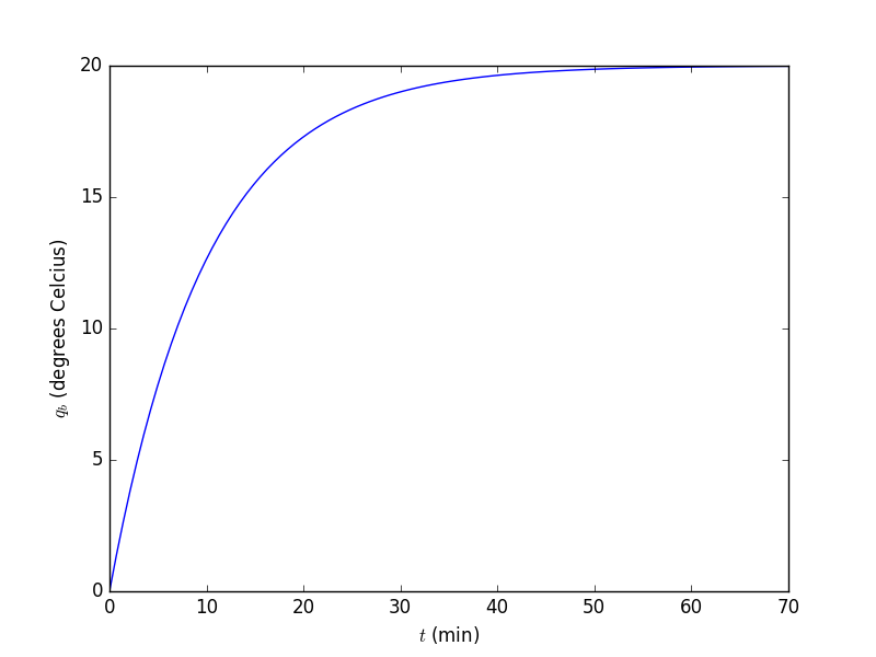
The surrounding temperature \(q_s\) is considered the input to the system and the temperature of the block \(q_b\) is the output of the system. When the surrounding temperature at time \(t=0\) jumps from zero degrees to 20 degrees we feed this termal system with a step function \(q_s(t)=20 u(t)\) where \(u(t)\) is the unit step function.

5.4.1.2. A Bumpy Road

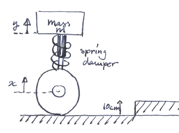
Car Suspension. Very much simplified as we look at one wheel only, and we neglect the suspension effect of the rubber tire itself.

The combination of a car equiped with shock absorbers is a nice example of a second order system. Consider just one wheel of the car with a shock absorber. The force exerted by the spring is proportional to its displacement: \(F_s=-k_s(y(t)-x(t))\). The force exerted by the damper is proportional to the relative velocity of both ends of the damper: \(F_d = -k_d(\dot{y}(t)-\dot{x}(t))\). Here we use the notation \(\dot{y}\) to denote the time derivative of signal \(y\). The total force \(F=F_s+F_d\) will move the mass \(m\) according to Newton’s law:

\[m\,\ddot{y}(t) = -k_s\,(y(t)-x(t)) - k_d\,(\dot{y}(t)-\dot{x}(t))\]

Rearranging terms we get:

\[m\,\ddot{y}(t) + k_d\,\dot{y}(t) + k_s\,y(t) = k_d\,\dot{x}(t) + k_s\,x(t)\]

Taking the Laplace transform of both sides we get:

\[m\, s^2\, Y(s) + k_d\, s\, Y(s) + k_s\, Y(s) = k_d\, s\, X(s) + k_s\, X(s)\]

Collecting terms we can write the transfer functions of this system as:

\[H(s) = \frac{Y(s)}{X(s)} = \frac{k_d\, s + k_s}{m\,s^2+k_d\,s + k_s}\]

This is a second order system with a zero in the transfer function. We can use the scipy.signal package for calculating and visualizing the step response of this system (where we set all our constants to 1).

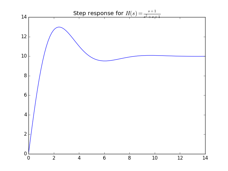
The step response of this system models what happens when you drive with your car on the sidewalk, suddenly your height is raised 10 cm. Due to the suspension (spring/damper system) your movement in the car is a bit more bumpy then the sudden jump. First you overshoot the sidewalk elevation of 10 cm and then you oscilate around that value before settling down to the 10 cm elevation.