4.2.8. Poles and Zeros

The generic form of the transfer function of a constant coefficient LTI system is:

\[H(z) = \frac{N(z)}{D(z)}\]

where \(N(z)\) and \(D(z)\) are polynomials in \(z\). Assuming \(M\)-th order polynomials we have:

\[H(z) = \frac{b_0 + b_1 z + b_2 z^2 + \cdots + b_M z^M}{ a_0 + a_1 z + a_2 z^2 + \cdots + a_M z^M}\]

In the complex domain a \(M\)-th order polynomial has exactly \(M\) zeros and we thus may write:

\[H(z) = K \frac{(z-z_1)(z-z_2)\cdots(z-z_M)}{ (z-p_1)(z-p_2)\cdots(z-p_M)}\]

where the zeros \(z_i\)‘s are the zeros of \(N(z)\) and the poles of the system, \(p_i\)‘s, are the zeros of \(D(z)\).

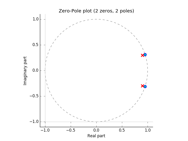
Because a LTI system is completely characterized by its transfer function \(H(z)\), the system is also completely characterized by its set of zeros and poles (together with a gain factor \(K\)). Plotting the zeros and poles in the complex plane gives the Argand diagram of the LTI system. In the Argand diagram we can also indicate the ROC of \(H(z)\).

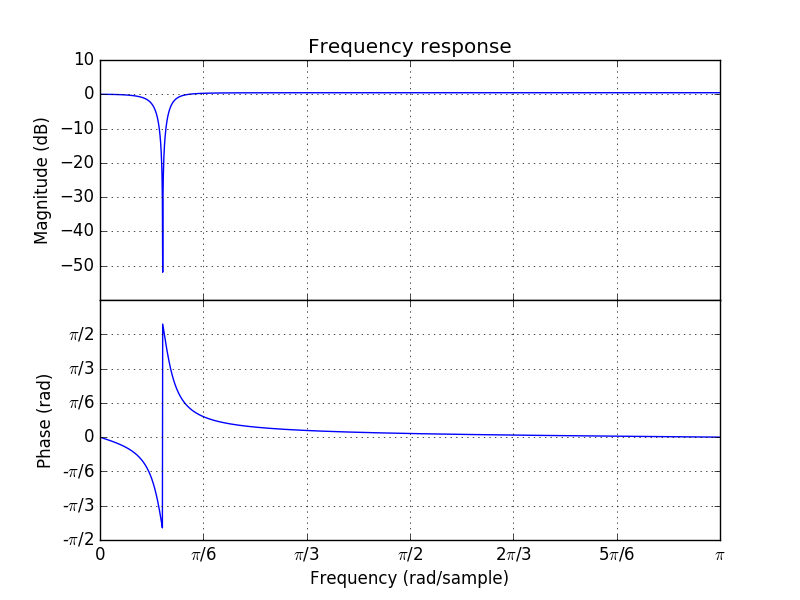
Consider the LTI system with transfer function \(H(z)\):

\[\begin{split}H(z) &= \frac{z^2 - 1.9 z + 1}{z^2 - 1.8 z + 0.9} \\ &= \frac{(z - 0.95 - 0.31j)(z - 0.95 + 0.31j)}{ (z - 0.9 - 0.3j)(z - 0.9 + 0.3 j)}\end{split}\]

The Argand diagram (plot of poles and zeros in the complex plane) and the frequency response \(H(e^{j\Omega})\) are sketched below (see later section on the \(\mathsf z\)-operator for the Python code).