3.1. Continuous Time Fourier Series
The CT Fourier Series considers periodic signals. A signal \(x(t)\) is periodic with period \(T\) in case:
Note that in case \(x\) is periodic with period \(T\) it is also periodic with period \(2T\) (or \(nT\)). This leads us to the definition of the fundamental period \(T_0\) being the smallest value such that \(x(t+T_0)=x(t)\). The fundamental frequency then is \(f_0=1/T_0\).
3.1.1. The Complex Exponential Functions
We have already introduced the complex exponential functions:
This funtion is periodic with period
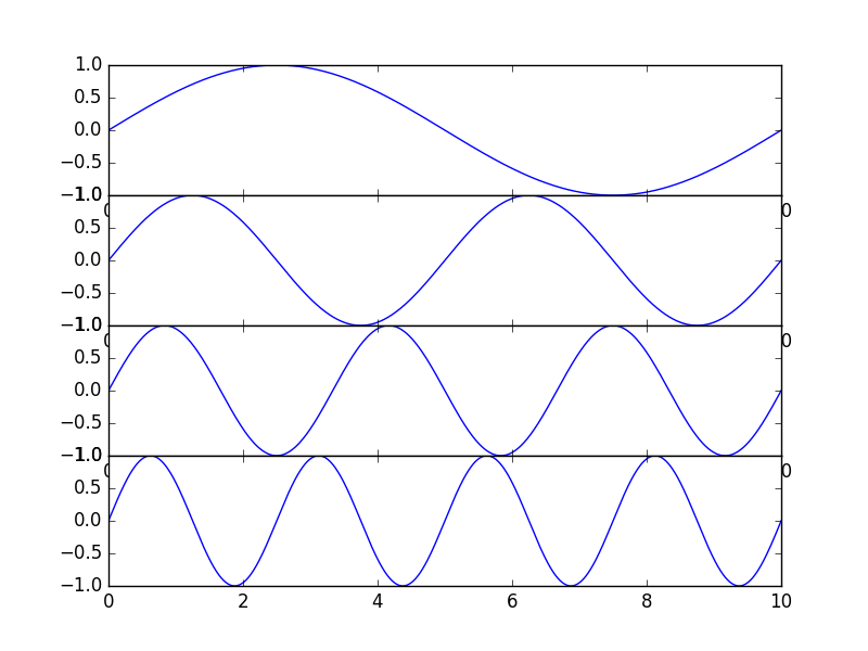
If we fix \(\omega\), say at value \(\omega_0\) then the fundamental period is \(T_0=2\pi/\omega_0\). The functions \(x(t)=\exp(j k\omega_0 t)\) for integer \(k>0\) then are all \(T_0\) periodic, in fact the fundamental period is:
Consider only the imaginary part of the complex exponential:
In [1]: from matplotlib.pylab import *

In [2]: T0 = 10

In [3]: t = linspace(0,T0,1000)

In [4]: for k in range(1,5):
   ...:     subplot(4,1,k)
   ...:     plot(t, sin(2*k*pi*t / T0))
   ...:

In [5]: show()
3.1.2. The Fourier Series
Fourier (a French mathematician) showed that nearly every periodic function (with period \(T_0\)) can be written as a linear combination (superposition) of the complex exponential functions \(\exp(j k \omega_0 t)\) for \(k=0,1,2,\cdots\) where \(\omega_0 = 2\pi / T_0\):
Note that the coefficients determining the weight of every frequency \(k\omega_0\) in general are complex valued.
The Fourier coefficients are given by:
Summarizing:
| Synthesis | Analysis |
|---|---|
\[x(t) = \sum_{k=-\infty}^{\infty} a_k e^{ j k \omega_0 t}\]
|
\[a_k = \frac{1}{T_0} \int_{\langle T_0 \rangle} x(t) e^{-j k \omega_0 t} dt\]
|
3.1.3. Properties I
In signal processing we are most often working with real valued signals. For such a real valued signal we have:
This is not too difficult to prove. First the synthesis equation can be rewritten such that we ‘unroll the summation loop’:
Using Eulers formula and writing \(a_k=A_k+jB_k\) where \(A_k\) and \(B_k\) are real numbers, we get:
Collecting real and imaginary parts leads to:
The imaginary part of the above equation can only be zero (what we need for a real signal) in case:
Both of these make \(a_{-k} = a^\star_k\).
So we can write:
Remember from high school trigonometry that a summation of a sine and cosine of the same frequency results in a shifted sine:
with the phase (shift) \(\phi\) given by:
This last synthesis equation shows that a periodic real valued function can be written as the sum of sine functions of frequency \(k\omega_0\) for \(k>0\).
For an even signal, i.e. \(x(-t)=x(t)\) we have:
For an odd signal, i.e. \(x(-t)=-x(t)\) we have:
3.1.4. Fourier Series Examples
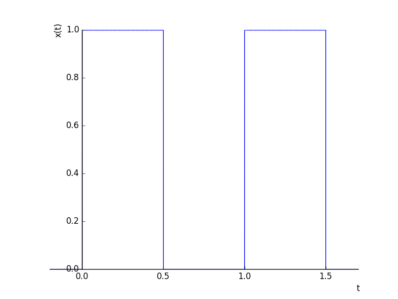
Showing examples requires the calculation of integrals in order to get at the values of \(a_k\) (the analysis equation). Most computer scientists are not that fond of integral calculations so we try to do it here using Sympy, a symbolic math package.
In [6]: import matplotlib.pylab as plt

In [7]: import sympy as sp

In [8]: t, T0 = sp.symbols("t, T0")

In [9]: x = sp.Piecewise(
   ...:        (1, t % T0<=T0/2),
   ...:        (0, True))
   ...:

In [10]: sp.plot(x.subs(T0,1), (t,-.2, 1.7), xlabel="t", ylabel="x(t)", line_width=3);

In [11]: plt.show()
Next we define a function that calculates the \(a_k\):
In [12]: import numpy as np

In [13]: def ak(k):
   ....:     return 1/1 * sp.integrate( x.subs(T0,1) * sp.exp(-1j * k * 2 * sp.pi / 1 * t), (t, 0, 1))
   ....:

#%timeit print(sp.N(ak(0))) # swwitched off because it takes around 30 s on my machine...
But this functions is very very slow... (probably due to the fact that the piecewise function makes integration hard when Sympy doesn’t recognize the fact that it just has to integrate the exponential function over half the period. Using this knowledge expicitly we get:
In [14]: import numpy as np

In [15]: def ak(k):
   ....:     return 1/1 * sp.integrate( sp.exp(-1j * k * 2 * sp.pi / 1 * t), (t, 0, 1/2))
   ....:

In [16]: for k in range(-5,6):
   ....:           print(k, sp.N(ak(k))) # almost instantanuous
   ....:
-5 -1.34748799232906e-27 + 0.0636619772367581*I
-4 -4.84464171678343e-134 + 0.e-128*I
-3 5.23500617355075e-27 + 0.106103295394597*I
-2 -4.84464171678343e-134 + 0.e-128*I
-1 -2.99311153379901e-27 + 0.318309886183791*I
0 0.500000000000000
1 -2.99311153379901e-27 - 0.318309886183791*I
2 -4.84464171678343e-134 - 0.e-128*I
3 5.23500617355075e-27 - 0.106103295394597*I
4 -4.84464171678343e-134 - 0.e-128*I
5 -1.34748799232906e-27 - 0.0636619772367581*I
3.1.5. Properties II
RVDB
Differentiation
3.1.6. Convergence of the Fourier Series
RVDB
- difference between point wise and integral (??) convergence
- Gibbs phenomenon