Dynamic modelling: Free fall

A dynamic model describes the behaviour of a system in time and is characterised by the¹

• initial state of the system;
• factors that influence the change of the state;
• time step in which the change takes place;
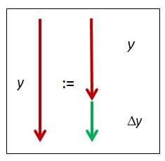
• recursive rule: new state := old state + change.

In the experiment to determine the acceleration of free fall, Table 1 provides a description of the falling motion divided into discrete time steps Δt. The state variables are the position y and the velocity v; change is determined by the gravitational acceleration g.

Based on the assumption that the acceleration of free fall is constant, Table 1 can be used to construct a dynamic model for computing the falling motion. In this model, the recursive rule for the compuration of the new state is

$$\begin{array}{l}v:=v+\Delta v\\ y:=y+\Delta y\end{array}$$

For given initial values of the position and the velocity, with these formulas, the falling motion of an object on which only the gravitational force works can be reconstructed step by step. With each subsequent time step, the change of position and velocity is computed and added to the previous state. The results can be compared with the measured data in Table 1.

Above, the transition actually takes place from the 'model of' free fall (Table 1) to a mathematical 'model for' free fall. For students, this is a big conceptual step that requires explicit attention in lessons. In textbooks, this conceptual step is often implicit in the explanation of the computational model of the motion of an object.²