2. Introduction to Python for Image Processing And Computer Vision
The combination of Python (the language), Numpy (the numerical array lib), SciPy (scientific libs) and Matplotlib (the graphical plot lib) will serve as our computational basis to learn image processing and computer vision. Where possible and needed we will use other libraries as well. We will use the name ‘Python’ to refer to this collection of tools.
The best way to explore Python is by using it. We assume that you have
ipython installed on your computer. All interaction shown is from
actual ipython sessions. Start ipython with the command
ipython.
You can start right away typing commands into the command line window:
The interpreter executes this statement and shows nothing (meaning
that there were no errors). We may look at the value of variable x
by just typing its name:
In [1]: x
Out[1]: 2
In Python there is no need to declare variables before using them.
If you start losing the overview over which variables you have already
used and which data they contain, the command whos can help you
out.
In [2]: whos
Variable   Type      Data/Info
------------------------------
np         module    <module 'numpy' from '/ho<...>kages/numpy/__init__.py'>
plt        module    <module 'matplotlib.pyplo<...>es/matplotlib/pyplot.py'>
x          int       2
In case you are not familiar with Python we suggest that you work your way through one of the tutorials that are available on the web (see some suggestions here).
In Python the list and dictionary are probably the most important datastructures. A list is a heterogeneous sequence of values (numbers, strings, lists, dictionaries, functions, really anything).
In [3]: a = [ 1, 2, 3, 4, 5 ]
In [4]: a[0]
Out[4]: 1
In [5]: a[3]
����������Out[5]: 4
In [6]: a[-1]
��������������������Out[6]: 5
Indexing is done using square brackets and indexing starts at 0. Negative indices start counting from the back to the front.
Using nested lists you may construct something that we would call a multidimensional list (or array) in C.
In [7]: a = [ [1,2,3], [4,5], [6] ]
In [8]: a[1]
Out[8]: [4, 5]
In [9]: len(a)
���������������Out[9]: 3
In [10]: len(a[1])
�������������������������Out[10]: 2
In [11]: a[0][1]
������������������������������������Out[11]: 2
But because of the list being heterogeneous and nested lists all can have their own length the list is not the preferred way to encode multidimensional arrays as the often are encountered in numerical computing.
The best way of learning Numpy is by reading the official tutorial: Tentative Numpy Tutorial.
2.1. Python for Image Processing
To demonstrate the use of Python for image processing we will look at two algorithms in some depth here: contrast stretching and linear filtering.
2.1.1. Contrast Stretching
Contrast stretching is described in histogramBasedOperations. Let \(f\) be a scalar image within the range \([0,1]\in\setR\). Then the contrast stretched image \(g\) is defined as:
Observe that this is a point-operator and we therefore do not need an explicit loop over all pixels (see Point Operators).
def cst( f ):
  fmin = amin(f) # the min value in an array
  fmax = amax(f) # the max value in an array
  return (f-fmin)/(fmax-fmin)
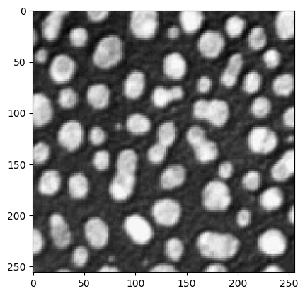
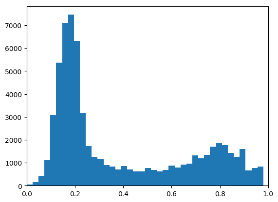
The image lowcontrast.npy uses
only part of the range from 0 to 1. Make an histogram of this image
and of the contrast stretched version of it.
The cst operator is so common when displaying images that it is even built into the matplotlib imshow function. For floating point images the values are always stretched to comprise the whole range from 0 to 1. To undo this automatic stretching in the imshow function you have to use something like:
In [12]: from pylab import *;

In [13]: a = imread("images/cermet.png");

In [14]: clf(); imshow(a,vmin=0,vmax=1,cmap=cm.gray);

In [15]: h, be = histogram(a.flatten(), bins=40)

In [16]: clf(); bar( be[0:-1], h, width=diff(be)[0] ); xlim( (0,1) );
Exercise:
Run your version of the cst algorithm on the lowcontrast.npy
image and plot its histogram.
2.1.2. Linear Filtering
With little doubt the linear filter is the most used filter in the image processing toolbox. It simply calculates a weighted summation of all pixel values in a small neighborhood (small compared to the image size). It does so for all shifted neighborhoods in an image and all weighted sums thus form a new image. In signal processing this would be called a moving (weighted) average filter.
Let \(F\) be the discrete function with all samples of the original image and let \(W\) be the weight function, the result image \(G\) then is called the correlation of \(F\) and \(W\):
Although there are built-in functions that calculate the linear filter efficiently, here we are showing a pure Python implementation. In the above mathematical expression we assumed the image (and weight function) to be infinitely large (hence the indices that run from \(-\infty\) to \(+\infty\)).
In practice we have to deal with the fact that the image is defined only on a finite domain. Then the indices \((i+l, j+l)\) can point outside the image (see the border problem) and we have to decide what value to use for \(F(i+k, j+l)\).
In practice the weight function has non zero values only in small neighborhood of the origin. Assume that \(W(k,l)\) is non zero only in the neighborhood for \(k=-K,..,+K\) and \(l=-L,..,+L\).
def linfilter1(f, w):
  g = empty(f.shape, dtype=f.dtype)  # the resulting image
  M,N = f.shape
  K,L = (array(w.shape)-1)//2

  def value(i,j):
    """The function returning the value f[i,j] in case
    (i,j) in an index 'in the image', otherwise it return 0"""
    if i<0 or i>=M or j<0 or j>=N:
      return 0
    return f[i,j]

  for j in range(N):
    for i in range(M):
      summed = 0
      for k in range(-K,K+1):
        for l in range(-L,L+1):
          summed += value(i+k,j+l) * w[k+K,l+L]
      g[i,j] = summed
  return g
Note that the correlation function linfilter1 has 4 nested
loops. For large images and large kernels it explains why even the
simplest image processing function are so processor intensive. Because
of the interpreted nature of the Python language writing a 4 levels
nested loop is bound to result in a very slow program. Test this
function on a small image.
In [17]: from linfilters import *;
In [18]: from scipy.ndimage.interpolation import zoom;
In [19]: from pylab import *; rcParams['savefig.bbox'] = 'tight'
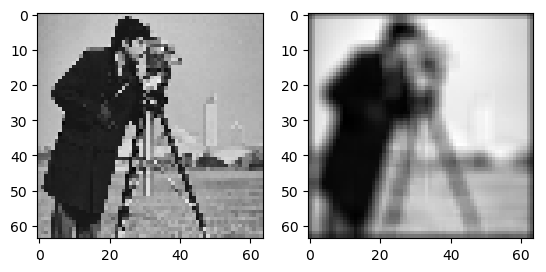
In [20]: a = imread('images/cameraman.png' );
In [21]: f = zoom(a, 0.25);
In [22]: g = linfilter1(f, ones((5,5))/25);
In [23]: subplot(1,2,1);
In [24]: imshow(f); gray();
In [25]: subplot(1,2,2);
In [26]: imshow(g);
Python doesn’t like expliciteloops (i.e. they are slow). In many cases we can come up with other ways to implement the same function and circumvent most explicit loops. Obviously the loops over all pixels and all neighbors must be there somewhere but ‘hidden’ in Python functions (written in C) and therefore we can achieve considerable speedups.
def linfilter2(f, w):
  """Linear Correlation based on neigborhood processing without loops"""
  g = empty(f.shape, dtype=f.dtype)
  M,N = f.shape
  K,L = (array(w.shape)-1)//2

  for j in range(N):
    for i in range(M):
      ii = minimum(M-1, maximum(0, arange(i-K, i+K+1)))
      jj = minimum(N-1, maximum(0, arange(j-L, j+L+1)))
      nbh = f[ ix_(ii,jj) ]
      g[i,j] = ( nbh * w ).sum()
  return g
This version circumvents the double loop over all pixels in the neighborhood. It extracts a detail image of the correct size. The correct multi-indices are build with the ix_ function.
Instead of ‘hiding’ the loops over all pixels in the neighborhood we can hide the loops over all pixels in the image. Observe that a correlation is equal to the addition of shifted and weighted images.
def linfilter3(f, w):
  """Linear Correlation using Translates of Images"""

  M,N = f.shape
  K,L = (array(w.shape)-1)//2

  di,dj = meshgrid(arange(-L,L+1), arange(-K,K+1))
  didjw = zip( di.flatten(), dj.flatten(), w.flatten() )

  def translate(di,dj):
    ii = minimum(M-1, maximum(0, di+arange(M)))
    jj = minimum(N-1, maximum(0, dj+arange(N)))
    return f[ ix_(ii, jj) ]

  r = 0*f;
  for di, dj, weight in didjw:
    r += weight*translate(di,dj)
  return r
And the easiest alternative is the builtin function correlate:
def linfilter4(f, w):
  return correlate(f, w, mode='nearest')
Exercise:
Time these alternatives using an image of size 64x64 for several sizes of the neighborhood (from 3x3 to 11x11 eg).
Make a plot with the timings as function of the neighborhood size for all filters.