2.1. Optic Flow

From Wikipedia:

Optical flow or optic flow is the pattern of apparent motion of objects, surfaces, and edges in a visual scene caused by the relative motion between an observer (an eye or a camera) and the scene.

The basic assumption used in most optic flow algorithms is that when a point \(\v x\) in the image at time \(t\) moves to point \(\v x + d\v x\) in the image at time \(t+dt\) its luminance does not change (the constant luminance assumption):

\[f(\v x+ d\v x, t+dt) = f(\v x, t)\]

Note that \(d\v x = \v v dt\) where \(\v v\) is the optic flow vector: the velocity vector at point \(\v x\) at time \(t\):

\[f(\v x + \v v dt, t+dt) = f(\v x, t)\]

because \(dt\) is assumed to be infinitessimally small we may approximate the above equations in first order as:

\[f(\v x, t) + (\nabla f)(\v x, t)\T \v v dt + f_t(\v x, t) dt = f(\v x, t)\]

or equivalently:

\[(\nabla f)(\v x, t)\T \v v + f_t(\v x, t) = 0\]

Note that given a video sequence \(f: (\v x, t) \mapsto f(\v x, t)\) we can approximate the spatial gradient \(\nabla f\) and the temporal derivative \(f_t\), but then we are left with just one equation and two unknowns: the two elements of the optic flow vector \(\v v\).

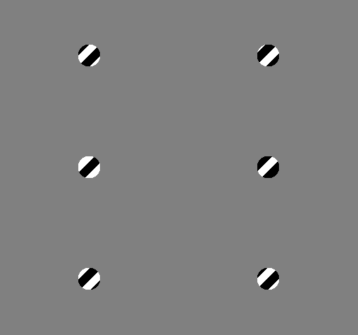
The impossibility to calculate the optic flow vector in a point is often called the aperture problem.

Fig. 2.6 From Wikipedia: The aperture problem. The grating appears to be moving down and to the right, perpendicular to the orientation of the bars. But it could be moving in many other directions, such as only down, or only to the right. It is impossible to determine unless the ends of the bars become visible in the aperture.

There are many known methods to circumvent the aperture problem (of course you cannot solve the ‘problem’, in fact to call it a problem is a bit of a misnomer). In these notes we consider only one: the Lucas and Kanada method.

The Lucas and Kanada method assumes that around a point \(\v x\) a lot of points in the neighborhood of \(\v x\) have the same optic flow vector \(\v v\). Let \(\v x_1,\ldots,\v x_n\) denote \(n\) points from the local neighborhood of \(\v x\). Then for all \(i=1,\ldots,n\):

\[(\nabla f)(\v x_i, t)\T \v v + f_t(\v x_i, t) = 0\]

or equivalently (using \(\v v = (u\;v)\T\)

\[f_x(\v x_i, t) u + f_y(\v x_i, t) v = - f_t(\v x_i, t)\]

Stacking all equations for \(i=1,\ldots,n\) we get:

\[\begin{split}\begin{pmatrix} f_x(\v x_1, t) & f_y(\v x_1, t)\\ f_x(\v x_2, t) & f_y(\v x_2, t)\\ \vdots \\ f_x(\v x_n, t) & f_y(\v x_n, t) \end{pmatrix} \begin{pmatrix}u\\v\end{pmatrix} &= - \begin{pmatrix} f_t(\v x_1, t)\\ f_t(\v x_2, t)\\ \vdots\\ f_t(\v x_2, t) \end{pmatrix}\\ A \v v &= -\v b\end{split}\]

In case we have more then two points (\(n>2\)) this is overdetermined system and we may solve it using a least squares procedure, leading to:

\[\v v = - (A\T A)\inv A\T \v b\]

The matrix \(A\T A\) is a \(2\times2\) matrix:

\[\begin{split}A\T A = \pmatrix{ \sum_{i=1}^n f_x^2(\v x_i, t) & \sum_{i=1}^n f_x(\v x_i, t) f_y(\v x_i, t) \\ \sum_{i=1}^n f_x(\v x_i, t) f_y(\v x_i, t) & \sum_{i=1}^n f_y^2(\v x_i, t) }\end{split}\]

and is commonly known as the structure tensor. Note that matrix \(A\) and thus also the structure tensor is dependent on the position in the image (we have taken \(\v x_i\) for \(i=1,\ldots,n\) to be points in the neighborhood of \(\v x\)).

When implementing this approach we have to consider:

• which neighborhood to choose and
• whether points in the neighborhood should be prioritized (weighted) when calculating the least squared error.

The Lucas-Kanade method to find the optic flow field (i.e. the flow vectors \(\v v\) for all positions in the image) is only valid for small discplacements (low velocity). For large displacements (more then say 2 pixels) the method cannot be used as such. However we could make an image pyramid such that large velocities are found from small displacements in subsampled images.