An Introduction to Local Structure in Scale-Space
When looking at pictures, even abstract depictions of things you have never seen before, you will find that your attention is drawn to certain local features: dots, lines, edges, crossings etc. In a sense there are ‘prototypical pieces’ of an image, and we can describe every image as a field of such local elements. You may group these into larger objects and recognize those, but viewed as a bottom-up process perception starts with local structure.
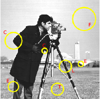
Local Image Structure. In an image we distinguish several types of local structure like constant patches (F), edges (E), lines (L), corners (C) etc.
Any visual perception system looking at the 3D world needs to address the task of size or scale invariance. The same object nearby will appear larger then the same object at larger distance and thus all local details will appear at varying sizes.
So when looking at local structure in images we have to
- define the notion of ‘local’, and
- define the notion of ‘structure’.
In our exposition of local image structure we adhere to linear scale space analysis as introduced by J.J. Koenderink in the 80ties of the 20th century.
Linear Gaussian Scale-Space
In the seminal paper on the ‘Structure of Images’ Jan Koenderink showed that the logical way to embed the original (primal) image \(f_0\) into a one parameter family of images where the parameter encodes the level of resolution (size of the details that can be distinguished) is the Gaussian convolution:
where \(G^s\) is the Gaussian function:
The 3D function \(f\) is called a scale-space as it explicitly encodes the scale. For any value of \(s>0\), \(f(\cdot,\cdot,s)\) is an image: a smoothed version of the original image. For \(s\downarrow0\) we have that \(f_0\ast G^s\rightarrow f_0\) and therefore we set \(f(\cdot,\cdot,0)=f_0\). For \(s\rightarrow\infty\) we are effectually at every point taking the weighted average of all function values, and thus for \(s\rightarrow\infty\) we have that \(f(\cdot,\cdot,s)\rightarrow\text{constant}\) with the constant equal to the average value of the original image.
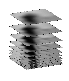
Gaussian Scale Space. visualized by a few images \(f(\cdot,\cdot,s)\) for different values of \(s\). The value of \(s\) increases going from the bottom to the top.
Koenderink came to this scale space construction by introducing the requirement of causality in scale space and showing that causasility is most easily met with using the Gaussian convolution to construct a scale-space. Causality is not enough to single out the Gaussian convolution, it is also assumed that the scale space operator is translation invariant (no preferred positions in the visual field), rotation invariant (no preferred directions) and most importantly it is assumed that the scale space operator is a linear operator.
Causality in scale space prevents the use of linear operators that do smooth the image but can introduce spurious detail at coarse scales that are not caused by structures at finer scales.
Properties of the Gaussian Convolution
The Gaussian kernel function used in a convolution has some very nice properties.
Separability
The property that is of great importance in practice is that is a separable function in the sense that we may write:
where \(G^s(x)\) and \(G^s(y)\) are Gaussian functions in one variable:
It is not hard to prove (starting from the definition of the convolution) that a separable kernel function leads to a separable convolution in the sense that we may first convolve along the rows with a one dimensional kernel function followed by a convolution along the columns of the image. The advantage is that for every pixel in the resulting image we have to consider far less values in the weighted sum then we would have to for a straightforward implementation.
Semi Group
If we take a Gaussian function \(G^s\) and convolve it with another Gaussian function \(G^t\) the result is a third Gaussian function:
From a practical point of view this is an important property as it allows the scale space to be build incrementally, i.e. we don’t have to run the convolution \(f_0\ast G^s\) for all values of \(s\). Say we have already calculated \(f(\cdot,\cdot,t) = f_0\ast G^t\), for \(t<s\), then using the associativity and the above property we have:
Note that \(\sqrt{s^2-t^2}<s\) and thus the above convolution will be faster then the convolution \(f_0\ast G^s\).
Smoothness and Differentiability
Let \(f_0\) be the ‘original’ image and let \(f(\cdot,\dot,s)\) be any image from the scale space (with \(s>0\)). Then no matter what function \(f_0\) is, the convolution with \(G^s\) will make into a function that is continuous and infinitely differentiable. Using Gaussian convolutions to construct a scale space thus safely allows us to use many of the mathematical tools we need (like differentation when we look at the characterization of local structure).
Sampling Scale Space
Spatial Sampling
Images are most often sampled equidistant in both directions, i.e. \(\Delta x=\Delta y\). The sampling distance is assumed to be chosen in relation to the smoothing introduced by the image acquisition and in accordance with the sampling theorem. We thus assume the original image is thus faithfully represented by its samples.
When constructing the scale space and thus smoothing the images with a Gaussian convolution we may use the fact that after smoothing we loose some high frequency details and thus we may subsample the image. This process of smoothing followed by subsampling is important in practice for efficiency reasons.
The original sampled image is not the ‘zero’ scale image (such a thing cannot exists as we always need measurement probes of finite size: pure point sampling is a physical impossibility). We assume the original image is smoothed at scale \(s_0=0.5\).
As we smooth the image in our scale space construction we loose some high frequency details and according to the sampling theorem we may subsample the image. Consider the image smoothed at scale \(s\), i.e. an observation scale that is \(s/s_0\) times as large as the original scale. Assuming the original image was correctly sampled we may subsample the image with the same factor. Assuming \(\Delta = \Delta x=\Delta y = 1\) for the original image we may choose:
for the sampling distance at scale \(s\). So in principle every image in the scale space could have a different number of pixels and still be a faithful sampling of the smoothed image.
Scale Sampling
Scale should be sampled logarithmically, let \(s_k\) for \(k=0,\ldots,K\) then we set
i.e. there is no constant difference between two scale samples but a constant ratio. The need for logarithmic sampling of the scale is intuively easy to see when you compare images in scale space. The larger the scale the more you have to smooth to see a noticible difference.
Choosing a value of \(\alpha\) depends on the purpose of the scale space construction. Choosing \(\alpha=2\) doubles the scale at every layer in the scale space. A lot of practical work has been done using such a course sampling (starting with a 1024x1024 image already after 10 smoothing steps the image is effectively reduced to a single pixel).
It has been shown that \(\alpha=2\) is to large in case we are looking for local structure in image, in such cases \(1<\alpha<2\) is more appropriate, typical choice then is \(\alpha\approx1.2\).
Scale Space Pyramids
Scale Space Stack
The simplest choice for constructing a scale space is to ignore the possibility of reducing the number of samples by subsampling the image. We then obtain a stack of images all of the same size but smoothed at different scales (logaritmically sampled of course).
Burt Pyramid
In the Burt pyramid (named after its inventor), the scale ratio \(\alpha=2\) is chosen. This means that after each smoothing step we may subsample the image with a factor 2. Assuming the original image is equal to \(s_0\), then after convolution we should get the image at scale \(s_1=2s_0\) therefore we need to convolve with \(G^{s_0\sqrt{3}}\). The image \(f(\cdot,2s_0)\) is then subsampled with a factor 2 (in all directions) i.e. \(\Delta = 2\).
To get from \(f(\cdot,2s_0)\) to \(f(\cdot,4s_0)\) we need to convolve with \(G^{2s_0\sqrt{3}}\). But in case we don’t convolve \(f(\cdot,2s_0)\) sampled on the original grid but on the subsampled grid with twice the sampling distance we have to convolve the subsampled image with \(G^{s_0\sqrt{3}}\), i.e. the same kernel we have used to get from \(s_0\) to \(2s_0\) working on the original image.
The same calculations can be made for all level in the pyramid. Every step involves: convolve with \(G^{s_0\sqrt{3}}\) and subsample by a factor of 2 in all directions.
Lowe Pyramid
Although the Burt pyramid has some very nice properties, it is not used much in scale space applications because the scale sampling is too coarse: we may loose details that have a size that is halfway inbetween two scale samples (say a feature of size \(6s_0\) which is inbetween the scales \(4s_0\) and \(8s_0\). In some cases interpolation cannot help us.
Recognizing that we need a finer sampling of the scale, but also recognizing the attrativity of the subsampling with a factor 2, Lowe introduced the concept of octaves in what i would like to call the Lowe Pyramid.
Lowe chooses an \(\alpha\) such that after \(L\) smoothing steps a doubling of the scale is achieved: \(\alpha^L=2\) or equivalently \(\alpha=2^{1/L}\).
A Lowe pyramid then first uses the original sampling resolution to do \(L\) smoothing steps (of which the last one brings the scale up to 2 times the original scale), then the image is subsampled and the procedure is repeated, keeping the sampling distance equal for \(L\) images and then subsample.
It can be shown that just as in the Burt pyramid (where there is only one image in each octave) the smoothing operators within one octave are the same for each of the octaves.
Lindenberg Pyramid
The Lindenberg pyramid is the most straightforward implementation of the idea that after smoothing and thereby increasing the scale from \(s_i\) to \(s_{i+1}=\alpha s_i\) we may enlarge the sampling distance with the factor \(\alpha\). Using an interpolation technique we are not dependent on the factor 2 subsampling in the Burt or Lowe pyramid.
Gaussian Derivatives
Derivatives are the mathematical language for change. Thus a theory that tries to characterize local structure which is all about the change in gray value in nearby points can use derivatives as a starting point. Furthermore for the description of the structure of smooth function surfaces differential geometry provides the mathematical tools. Thus in selecting derivatives as a starting point in the description of local image structure allows us to tap into a vast body of knowledge and tools.
In case your calculus course was a long time ago you might want to take a quick look at a short recap of math for multivariate functions.
Locally a function can be approximated with the Taylor expansion of the image function. Consider the image function \(f\) and consider the second order Taylor expansion around a point \((a,b)\):
In the above we have used the notation that \(f_x\) is the first order derivative of \(f\) in its first argument (with respect to \(x\)). Equivalently \(f_{xy}\) is the mixed derivative (one time with respect to \(x\) and one time with respect to \(y\)). We may safely assume that all the derivatives do exist as all the functions we will be differentiating are smooth in the mathematical sense (i.e. all order derivatives do exist) because we will be looking at the derivatives of a Gaussian smoothed image.
Given the 6 values \(f(a,b)\), \(f_x(a,b)\), \(f_y(a,b)\), \(f_{xx}(a,b)\), \(f_{xy}(a,b)\) and \(f_{yy}(a,b)\) we can approximate the function \(f\) in the neighborhood of \((a,b)\). The derivatives thus characterize the function and we therefore should be able to characterize local structure using only the derivatives. Using only the derivatives up to order 2 (as done in the above Taylor expansion) it is impossible to characterize structure that is more complex then simple edges, corners and line like structure.
Higher order Taylor expansions and thus higher order derivatives can be used to characterize more complex structure. In this introduction we stick to the second order Taylor models as higher order models require more math (tensor calculus).
In a later section we are going to use the Gaussian derivatives to construct detectors for specific details in images (edges, lines and corners). First we look at the way derivatives behave in scale space and in what way we can calculate derivatives of sampled functions.
Derivatives in Scale Space
Taking a derivative of a function (any order) is a linear operator, furthermore it is a translation invariant operator. Therefore the derivative operator commutes with any convolution (see the section on linear operators). I.e. taking the derivative of convolved function is the same as convolving the derivative of the function. Let \(\partial_\ldots\) denote any derivative operator (of any order and in any set of variables), we have that
This shows that the derivatives of a function (image) are smoothed in the same way in linear scale space.
Calculating Derivatives of Sampled Functions
Building a model for local image structure based on calculating derivatives was considered a dangerous thing to do in the early days of image processing. And indeed derivatives are notoriously difficult to estimate for sampled functions. Remember the definition of the first order derivative of a function \(f\) in one variable:
Calculating a derivative requires a limit where the distance between two points (\(x\) and \(x+dx\) is made smaller and smaller. This of course is not possible directly when we look at sampled images. We then have to use interpolation techniques to come up with an analytical function that fits the samples and whose derivative can be calculated.
In Gaussian scale space we can combine the smoothing, i.e. convolution with a Gaussian function, and taking the derivative. Let \(\partial\) denote any derivative we want to calculate of the smoothed image: \(\partial(f\ast G^s)\). We may write:
Even if the image \(f\) is a sampled image, say \(F\) then we can sample \(\partial G^s\) and use that as a convolution kernel in a discrete convolution.
Note that the Gaussian function has a value greater than zero on its entire domain. Thus in the convolution sum we theoretically have to use all values in the entire image to calculate the result in every point. This would make for a very slow convolution operator. Fortunately the exponential function for negative arguments approaches zero very quickly and thus we may truncate the function for points far from the origin. It is customary to choose a truncation point at about \(3s\).
Local Structure
We have thusfar only stated that we can characterize local structure using the image derivatives. In this section we give some examples. For a more detailed explanation we refer to the more detailed section on local structure.
Canny Edge Detector
An edge delineates transition from dark to bright regions in an image. Consider a univariate function \(f\) in \(x\) showing a transition from low to high values and its first order derivative \(f'=f_x\) and second order derivative \(f''=f_{xx}\).
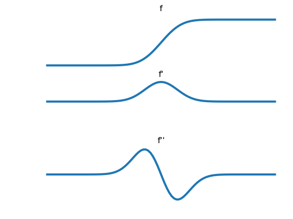
We see that the first order derivative peaks at the position of the edge (the point of maximal slope) and that the second order derivative crosses the zero level precisely at the point of maximal slope. Thus we may characterize an edge with the two conditions:
We can use this model for an edge in 2D as well, the only thing we then have to do is decide for every point in the image in which direction to look for an edge.
The gradient vector (see the chapter on local structure) is the vector
this gradient vector always points in the direction of maximal increase in gray value (think of yourself standing on a smooth mountain landscape, then there is always one unique direction in which the slope upwards is steepest: that’s the gradient direction). The gradient direction is obviously the direction to look for the edge.
The gradient direction is often called the \(w\) direction and thus the expression for the edge detector in images is:
i.e. the first order derivative
Note that the \(w\) direction varies from position to position in images.
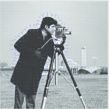
Gradient Vectors. The gradient vectors in many points in the image is plotted. Note that the gradient is perpendicular to the edges and is pointing in the direction of the maximal increase of gray value. The length of the gradient vector equals the first order derivative in the gradient direction (i.e. \(f_w = \sqrt{f_x^2+f_y^2}\)).
The results of selecting the points in an image that satisfy both conditions of the Canny edge detector are shown in the figures below. Note that we can calculate the edges for any scale \(s\) using Gaussian derivatives. Below we give the results for two scales.
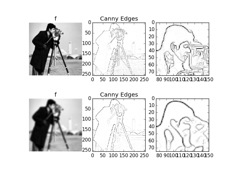
Canny Edge Detector working at two scales
Detectors based on Differential Geometry
Besides the Canny edge detector various other detectors for local structure can be build. We illustrate just a few of them:
Corner Detector
A corner detector looks for those locations in an image where a corner is visible. The simplest detector calculates the curvature (the bending) of isophotes (edges), the sharped the bend the more it looks like a corner. This can be proven to be proportional to the second order derivative in the \(v\)-direction (the direction perpendicular to the \(w\) direction).
Original Corners (scale = 2) Corners (scale = 3) Corners (scale = 5) 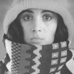
The bright spots indicate corners where the bright side of the object is ‘in the corner’, whereas the dark spots indicate the corners where the bright side of the object is ‘outside of the corner’.
Line Detector
The midpoint of line line structures (note that we cannot observe mathematical lines, here we mean lines with finite thickness) is a point where often the gradient vector vanishes (has length zero). In such cases the \(v\) and \(w\) directions are not defined.
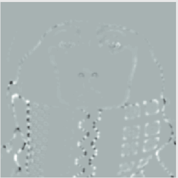
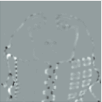
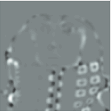
Original image Surface view of detail of image Detected lines 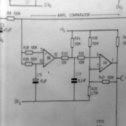
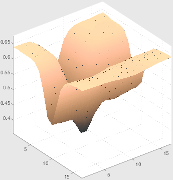
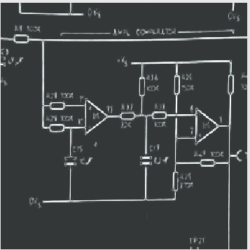
In the figure above on the ledt the original image is shown and on the right a surface view of the gray value function. The details shows the gray value function at the position of a line junction.
In such case we may look at he second order structure of the image, i.e. the way the image function is ‘curved’. A detector for lines can then be build based on the value of the second order derivatives.
T-Junction Detector
When looking at one object that is partly hidden by an object in front of it the observer will see T-junctions. These junctions require 3rd order derivatives to detect.
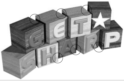
T-junctions detector.
T-junctions often emerge at occlusion boundaries. The foreground edge is most likely to be the straight edge of the “T”, with the occluded edge at some angle to it. The circles indicate some T-junctions in the image. (image taken from book of B. ter Haar Romeny)
Histogram of Gradients
The previous examples have shown several examples of local structure detectors that are based on differential geometrical reasoning. Although a very powerfull technique nowadays we more often find that local structure descriptors are not constructed from carefull differential geometrical reasoning but from simple statistics and machine learning techniques.
It can already be traced back to the writings of Koenderink who indicated that instead of describing complex structure with high order derivatives it also possible to describe the same structure as a spatial combination of less complex (i.e. lower order differential structure). The spatial relations are then often not explicitly modelled geometrically but the structure is learned from experience (examples) using machine learning techniques.
The most famous example perhaps is the histogram of gradients descriptor as introduced by David Lowe in his seminal paper on the scale invariant feature transforms (SIFT). In this approach for local structure description we look at a point in an image and a neighborhood around it. This neighborhood is subdivided in several subregions (usually a 4x4 grid of square regions instead of the 2x2 grid in the figure below) and in each of the subregions a histogram of the gradient direction is calculated. Only 8 bins are chosen to make a histogram of orientations (ranging from 0 to \(2\pi\) degrees). The 16 histograms of all the histograms of the subregions are concatenated to form a 128 dimensional vector that numerically characterizes the neighborhood.
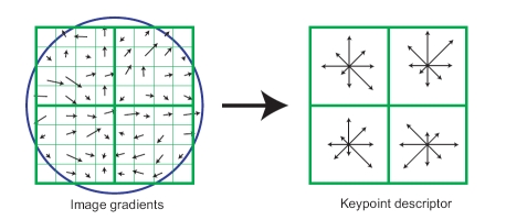
Around the center point a 2x2 grid of square regions is selected. For each subregion a histogram of the gradient directions is made, the concatenation of these histograms form the descriptor associated with the center point.
There are two scales hidden in this descriptor. The ‘inner’ scale, the scale at which the gradient vectors are calculated and the scale that determines the size of the neighborhood. Calculating such a descriptor for all possible scales of the neighborhood is usually too much work. Most often a technique to automatically select an appropriate scale is used. The scale selection technique that is at the heart of most practical applications is discussed in the next section.
It is somewhat surprising that such a ‘simple’ descriptor as the histogram of gradients proves to be so powerful in many practical applications.
Scale Selection
We started this introduction of local structure in scale space by introducing the Gaussian scale space as a way to record an image at all levels of resolution simultaneously. When we looked at local structure we showed example of local structure detected at one or several selected scales.
This section considers the task of automatically selecting the appropriate scale of looking at a point in an image. In this section we will look at the scale selection technique that is capable of selecting the position and size of a ‘blob’ in the image.
A blob is a bright circular shaped spot on a dark background (or a dark spot on a bright background).
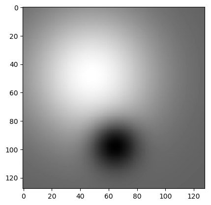
In the above image two ideal blobs are shown, a bright large blob in the top left and a dark smaller blob at the bottom center. An example of a natural image showing a lot of blobs at various scales is shown below. Every sunflower looks like a dark blob on a brighter background.
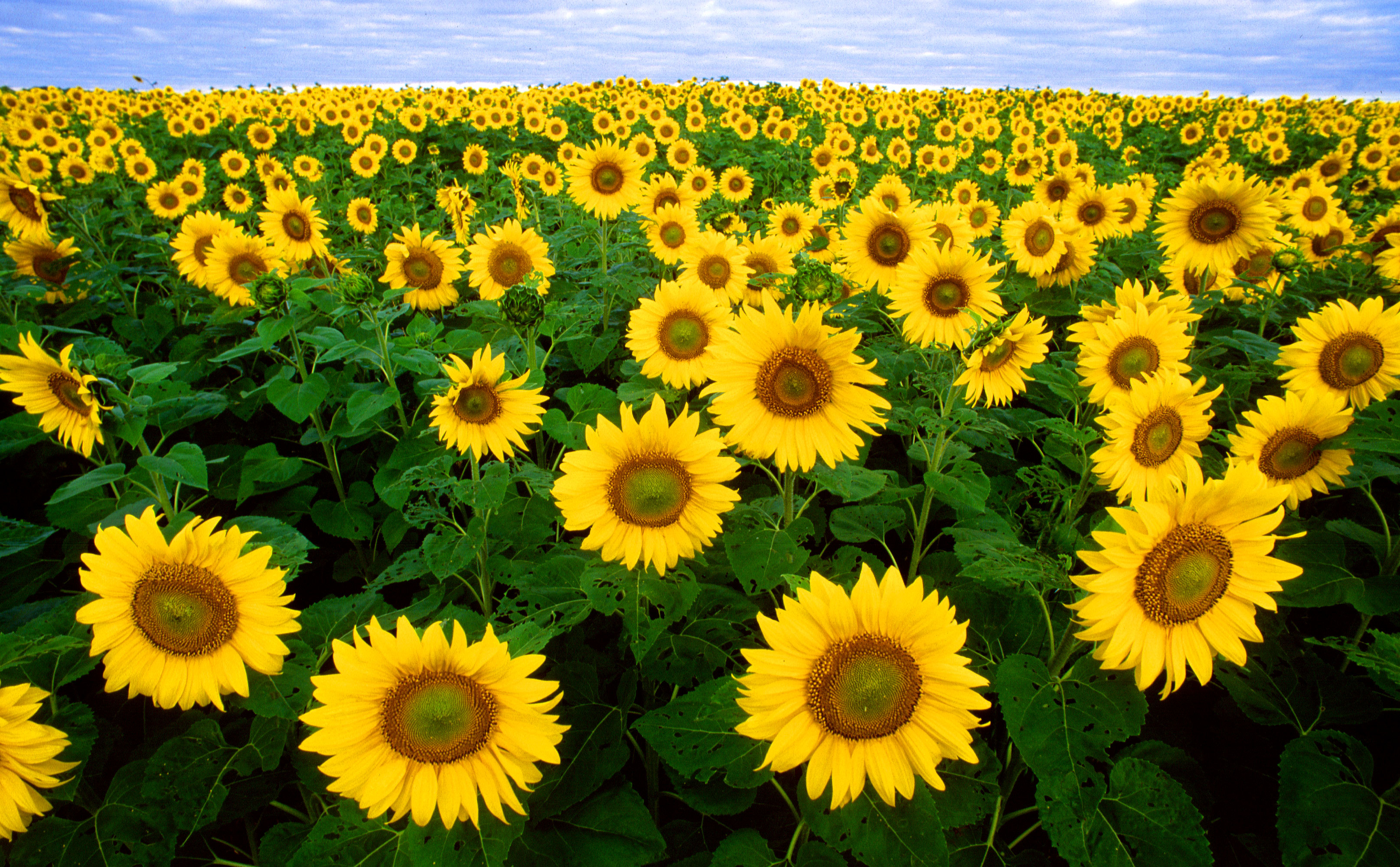
Blobs in natural images. Every sunflower is a dark blob on a bright background.
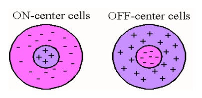
Center Surround Receptive Fields.
Detecting blobs with the Laplacian operator is very much like the use of center surround receptive fields in human vision. These receptive fields become active in case the center receives a lot of light and the surround far less light (or vice versa).
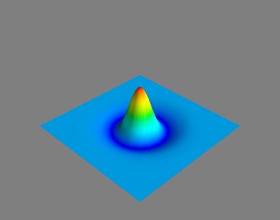
Laplacian or Mexican Hat. A surface plot of \(-\nabla^2 G^s\) is shown.
If we look at the Laplacian kernel function \(s^2\nabla G^s\) the similarity with a center surround receptive field is clear.
Finding blobs in scale space has been studied by T. Lindenberg. If we model blobs as shfted Gaussian functions (both positive and negative) as are shown in the first figure of this section, Lindenberg showed that we can locate these blobs in scale space by looking for the extremes of the scale space Laplacian:
where \(\nabla^2\) is the Laplacian operator:
It is not difficult to prove that in case at position \((x_0,y_0)\) a Gaussian blob of scale \(t\) is visible, then \(\ell(x,y,s)\) has an extreme value in \((x_0,y_0,s_0)\).
Blob detection in scale space then amounts to:
- calculate the Laplacian scale space \(\ell\), and
- find the scale-space points \((x,y,s)\) where \(\ell\) has an extreme value.
Finding an extreme value in a sampled scale-space is not trivial. In practice subpixel accurate localization is important and therefore interpolation techniques are required.
Although this technique is developed to find blobs, in a lot practical situations (e.g. SIFT) it is used to find keypoints in an image. Locally at the scale of the detected blob there is not much to see (by definition!) and therefore these applications first find the blobs using the scale selection mechanism described in this subsection. Then for a blob at scale-space location \((x,y,s)\) a much larger neighborhood (say of size \(3s\)) is used to calculate a histogram of gradients as a local structure descriptor.