Causality in Scale Space
In the seminal paper introducing linear scale space based on first principles in the western world (in the nineties of the 20th century it became clear that scale space was already invented in the sixties in Japan) J.J. Koenderink did not start with the principles of invariance. Instead he stated that a scale space should be causal in the sense that when going from small scales (high resolution) to large scales (low resolution) no new details (spurious details) will be introduced. The blurring involved in smoothing the image should only destroy structure and not introduce new structure.
Koenderink was looking for a linear operator \(\op L^t\) to make a scale space being a one parameter family of images \(f(\v x, t) = (\op L^t f)(\v x)\) with \(f(\v x, 0) = f_0\) where \(f_0\) is the zero-scale or original image.
Here we will not redo the proof of Koenderink, instead we will do a much simpler proof for a one dimensional ‘image’. So we are looking for a linear operator \(\op L^t\) that leads to the scale space \(f(x,t)=(\op L^t f)(x)\).
Causality as defined by Koenderink states that the change in value \(f\) at position \(x\) when going from scale \(t\) to scale \(t+dt\) (an infinitesimal small increase in scale) is caused by the image at scale \(s\). So there must exist an operator that takes the image at scale \(t\) and produces an image at scale \(t+dt\). Causality furthermore implies that for all points \((x,t)\) in scale space there must be a point \(y\) in the infinitesimal small neighborhood of \(x\) at an infinitesimal smaller scale \(t-dt\) such that \(f(x+dx,t-dt)=f(x,s)\). This is an asymmetric condition as we take \(dt>0\) whereas \(dx\) may be either positive or negative. What type of linear operator then satisfies the condition of causality?
Consider the curves in scale space (i.e. \((x,t)\)-space) where \(f(x,t)=\mbox{constant}\). Consider a point \((x_0,t_0)\) on such ‘isophote’.
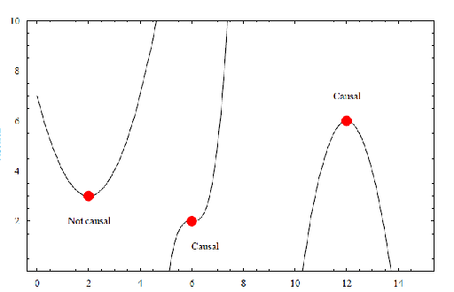
Isophotes in scale-space. On the horizontal axis is the spatial variable \(x\) and on the vertical axis is the scale \(t\).
Observe that only in case the isophote has a zero slope (i.e. horizontal tangent line) in point \((x,t)\) this point might violate the causality constraint. For all other points on a isophote there is a point \(x+dx\) at infinitesimal smaller scale \(t-dt\) which is also on the isophote.
So the important points to look at are the points where \(f_x(x)=0\) (note that we use the notation \(f_x\) to denote the partial derivative of \(f\) with respect to \(x\)), these are the stationary points. At these points the isophote can be parametrized as the function \(t=T(x)\) and we have \(f(x,T(x)) = \mbox{constant}\). Let \((x_0,t_0)\) be a stationary point on the isophote. At a stationary point we have \(T'(x_0)=0\) and it is the sign of \(T''(x_0)\) that determines whether the isophote satisfies the principle of causality or not. In case \(T'(x_0)<0\) the isophote locally looks like a parabole with the top facing up and thus the value \(f(x_0,t_0)\) can be found in a closeby point on a infinitesimally smaller scale. However in case \(T''(x_0)>0\) the isophote is a parabola with the top facing down and thereby violating the causality principle.
How to calculate \(T''\) then? We start with the defining equation:
If we now take the derivative with respect to \(x\) we get:
Repeating this:
We are only interested in \(T''(x_0)\) and knowing that \(T'(x_0)=0\) we find:
or equivalently
Causality in scale space requires that \(T''<0\) and thus
for any function \(\alpha\). Because there is no a priory preference for either position nor scale Koenderink decides to set \(\alpha=1\). This leads to the well known heat equation (i.e. a diffusion equation for constant diffusion coefficient, see wikipedia):
Given the initial condition \(f(x,t=0) = f_0(x)\) it is known that this partial differential equation is solved by
with
Note that \(g^t = G^s\) for \(s=\sqrt{2 t}\), thus indeed scale space has to be calculated as a Gaussian convolution of the original image. The difference is only a reparameterization of the scale.
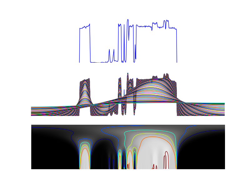
One Dimensional Scale Space. At the top the original 1D function \(f(x,0)\) is shown. In the center the original function and a smoothed images \(f(x,t)\) for a lot of values of \(t\) (logarithmically sampled) are shown until almost the constant value function is reached. At the bottom the scale-space function \(f(x,t)\) is depicted as an image. Horizontally the \(x\), vertically the \(t\) coordinate. The gray value at point \((x,t)\) is proportional to \(f(x,t)\). In this image some of the isophotes in scale space are shown.
Note that the ‘proof’ given in this section only looks at 1D functions (and thus a 2D scale-space). The proof in 2D is much more complicated due to the fact that \(f(x,y,t)=\mbox{constant}\) is a surface in 3D space and we need differential geometry to look for the stationary points and the causality condition.
In 2D the result is the partial differential equation:
which is solved with
with