7.2. k-Means, towards Gaussian Mixture Models

We start with a simple extension of the k-means algorithm in order to deal with spherical blobs of varying size. This is done by keeping track of the ‘variance’

\[\sigma_j^2 = \frac{1}{m_j} \sum_{i:c_i=j} \|\v x\ls i - \v\mu_j\|^2\]

and measuring the distance of a point \(\v x\ls i\) to a cluster \(\v\mu_j\) relative to the variance:

\[c_i = \arg\min_{j} \frac{\|\v x\ls i - \v\mu_j\|}{\sigma_j}\]

With this variance weighted distance measure the distance to a cluster center is effictively measured with a ruler for which the unit length is equal to the standard deviation of that cluster of points. The clustering of the 5 datasets is depicted below in Fig. 7.2.1.

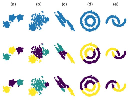
Fig. 7.2.1 k-Means Variance Clustering. For the first three datasets \(k=3\) is selected and for the last two datasets we have set \(k=2\). On the first row the original data sets. On the second row the k-means clustering results and on row 3 the results from the variance weighted k-means clustering.

From the figure it is clear that variance weighted k-means is better suited to deal with spherical clusters of different sizes. But still it can’t make sense of the ellipsoidal clusters in the 3rd column.

To deal with these ellipsoidal shaped clusters we will calculate the covariance matrix for each of the classes:

\[\Sigma_j = \frac{1}{m_j} \sum_{i:c_i=j} (\v x\ls i - \v\mu_j)(\v x\ls i - \v\mu_j)\T\]

and use the (squared) Mahalanobis distance for the label assignment:

\[c_i = \arg\min_j (\v x\ls i - \v\mu_j)\T \Sigma_j\inv (\v x\ls i - \v\mu_j)\]

where

\[d_M(\v x) = \sqrt{(\v x-\v\mu)\T \Sigma\inv (\v x-\v\mu)}\]

is the Mahalanobis distance from a point \(\v x\) to the distribution with mean \(\v\mu\) and covariance matrix \(\Sigma\). Note that for a scalar \(x\) and distribution with mean \(\mu\) and variance \(\sigma^2\) the Mahalanobis distance is equal to the distance measure where the length of the difference is divided by the standard deviation (as used at the start of this section).

The Mahalanobis distance generalises this idea of using the variances (in each direction) as yardstick. That is we measure distance in terms of how many standard deviations point \(\v x\) is away from the center of the distribution. Thus we take the ‘shape’ of the distribution into account.

Using the Mahalanobis distance will correctly cluster the data set in column (c) in Fig. 7.2.1. But will not deal with the data sets in the last two columns. Other ways of clustering are needed in these cases.

Clustering can be taken one (large) step further by using a Gaussian mixture model (GMM). In a GMM not only the Mahalanobis distance is estimated and used as a distance measure but the assignment to a cluster is not ‘hard’ (in the sense that the closest cluster wins) but ‘soft’ in the sense that each point is assigned to each cluster with a ‘strength’ that is inversely proportional to its distance to that cluster center.

A detailed description of the GMM is outside the scope of these lecture notes.