5.1.2. Multivariate Linear Regression

5.1.2.1. From 1 to \(n\) Features

Now suppose we have not one feature value \(x\) but \(n\) feature values \(x_1,\ldots,x_n\). We collect these values in a feature vector \(\v x = (x_1\ldots x_n)\T\).

Now the target value \(y\) depends on all these \(n\) values and a simple linear model is:

\[h_{\v\theta}(x_1, x_2, \ldots, x_n) = \theta_0 + \theta_1 x_1 + \cdots + \theta_n x_n\]

Again we augment our feature vector to deal with the bias term \(\theta_0\):

\[\begin{split}\hv x = \matvec{c}{1\\ \v x} = \matvec{c}{1\\ x_1 \\ \vdots\\ x_n}\end{split}\]

Convince yourself that from here it is downhill and completely as we have seen in the univariate case. The cost function is:

\[J(\v \theta) = \frac{1}{2m} \| \hv X \v \theta - \v y \|^2\]

and the gradient vector is:

\[\frac{\partial J(\v\theta)}{\partial \v\theta} = \frac{1}{m} \hv X\T (\hv X \v\theta - \v y)\]

Note that the increased complexity with respect to the univariate case is completely ‘hidden’ in the dimensions of the vector \(\v\theta\) and the matrix \(\hv X\).

5.1.2.2. Extended Features

Evidently not all functions that we would like to learn using a regression technique are linear in the data values. A standard way is to use an extended feature set. Let’s consider the univariate case again. Instead of only considering the value of \(x\) in a linear model we now add ‘new’ feature values. For instance we generate the augmented feature vector \(\hv x\):

\[\begin{split}\hv x = \matvec{c}{1 \\ x \\ x^2 \\ x^3}\end{split}\]

And again computationally not much changes: the cost function is the same and the gradient vector is the same (albeit with other dimensions of the data matrix \(\hv X\) and parameter vector \(\v\theta\).

Note that we are not restricted to the monomials as feature values. Consider a sinussoidal function \(a + b\sin(2x + c)\) where \(a\), \(b\) and \(c\) are parameters of our model (we assume that the frequency is known). The function as defined in this way is not suitable for linear regression (why not?). We therefore write:

\[h_{\v\theta}(x) = A + B \sin(2 x) + C \cos(2 x)\]

as an equivalent expression. In the following figures we show a data set that van be modelled with the above hypothesis but is corrupted by noise. Using linear reqression (we use the analytical solution in the code but could have equally well use the gradient descent procedure) we estimate the parameters \(A\), \(B\) and \(C\) and plot the learned model and compare with it with the ‘ground truth’ (possible because we have generated the noisy data ourselves).

In [1]: from matplotlib.pylab import *

In [2]: x = 10 * random_sample(50)

In [3]: xx = linspace(0,10,1000)

In [4]: x = sort(x)

In [5]: def generatey(x):
   ...:     return 5 + 3 * sin(2 * x + pi/3)
   ...: 

In [6]: yt = generatey(x)

In [7]: y = yt + 0.9 * randn(*x.shape)

In [8]: subplot(2,1,1);

In [9]: plot(x, y, '.');

In [10]: plot(xx, generatey(xx));

In [11]: tmp = (ones_like(x), sin(2*x), cos(2*x))

In [12]: X = vstack(tmp).T

In [13]: p = inv(X.T @ X) @ X.T @ y

In [14]: subplot(2,1,2);

In [15]: plot(xx, generatey(xx), 'g');

In [16]: def model(x, p):
   ....:     return p[0] + p[1] * sin(2*x) + p[2] * cos(2*x)
   ....: 

In [17]: plot(xx, model(xx,p) , 'b');

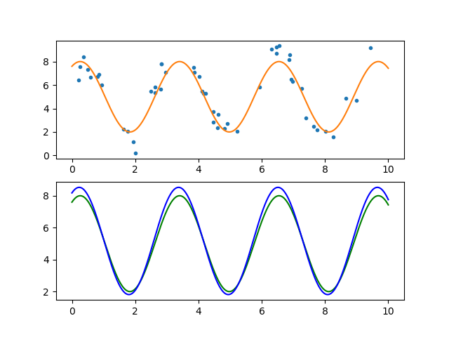
Observe that we only need 50 learning examples to get a fairly accurate estimation of the model parameters. This is only true in general in case the data is modelled accurately by the selected hypothesis function and the noise (deviations from the model) can be accurately described as additive normally distributed. In the last section of the Regression chapter we will derive the univariate regression algorithm from basic principles.