5.1.3. Dealing with Overfitting using Regularization

Consider the hypothesis function:

\[h_{\v\theta} = \theta_0 + \theta_1 x + \theta_2 x^2 + \cdots \theta_n x^n\]

We like to find the parameter vector \(\v\theta = (\theta_0\;\theta_1\;\cdots\;\theta_n)\T\) such that \(h_{\v\theta}\) fits the data points given below in the figure. Note that the ‘true’ function is depicted with a gray line.

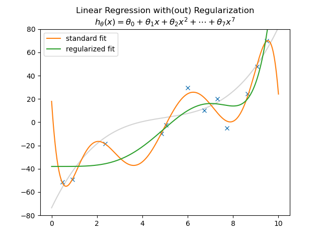
The standard linear regression function is plotted in orange. Because the model is too complicated for the data it will overfit. The model will do well on the learning set but will perform poorly on the test set.

Instead of selecting a less complex model (e.g. a lower order polynomial) we can use regularization. The regularization approach is based on the observation that the parameters of an overfitted model tend to get large. We then try to keep the parameters small by penalizing large parameters. This is done by adding a term to the cost function:

\[J(\v\theta) = \frac{1}{2m}\|\hv X\v\theta - \ \v y\|^2 + \frac{\lambda}{2m} \sum_{i=1}^n \theta_i^2\]

where \(\lambda\) is the regularization parameter that determines the relative importance of the regularization cost with respect to the fitting cost. Note that the \(\theta_0\), the bias parameter, is not taken into account in calculating the regularization cost.

For \(\lambda=0\) there is no regularization and we end up with the classic linear regression solution. For \(\lambda\rightarrow\infty\) regularization dominates completely and all parameters, except \(\theta_0\) will be zero.

Introducing the matrix:

\[\begin{split}D_0 = \begin{pmatrix} 0 & 0 & 0 & \cdots & 0\\ 0 & 1 & 0 & \cdots & 0\\ 0 & 0 & 1 & \cdots & 0\\ \vdots & \vdots & \vdots & \ddots & \vdots\\ 0 & 0 & 0 & \cdots & 1 \end{pmatrix}\end{split}\]

we can write:

\[J(\v\theta) = \frac{1}{2m}\|\hv X\v\theta - \v y\|^2 + \ \frac{\lambda}{2m} \| D_0 \v\theta \|^2\]

The gradient then becomes:

\[\pfrac{J(\v\theta)}{\v\theta} = \frac{1}{m}\hv X\T(\hv X\v\theta-\v y) + \ \frac{\lambda}{m}D_0 \v\theta\]

With this new gradient vector finding the optimal parameter vector is done in the same way as before. Start at a random initial vector and do the gradient descent iteration.

In the figure above besides the standard (unregularized) fit (in orange) also the regularized fit (in green) is shown.

The regularization parameter \(\lambda\) is a so called meta parameter. It is not a real parameter of the model itself, but it is a parameter of the cost function. Selecting the best regularization parameter requires ‘learning’ too. The learning procedure then is:

1. Divide your set of examples \(\{\v x\ls i, y\ls i\}\) into three parts: the learning set, the test set and the cross validation set.

2. For several values, say \(N\), of the meta parameter \(\lambda\) learn the model on the learning set. This results in \(N\) possibly different models (parameter vectors \(\v\theta\)).

3. Select the best out of the \(N\) models using the results based on the cross validation set.

4. Test this model on the test set to find the accuracy of your model.