This model forms the basis of the step-by-step calculation of movements, originally conceived by Isaac Newton. The calculation rule for uniform motion is that the new value for the position is given by the previous value plus the change in the time step \( \Delta t \).
4. Overview of models and model equations
4.1 Force and motion
Modelling is introduced in many textbooks in the subject of Force and Motion.1 Students are familiar with motion and its graphical representations through lessons on kinematics. This allows them to interpret and assess graphs that are the outcomes of modelling tasks. In addition, quantities such as velocity and acceleration indicate a change; that makes it easier for students to accept the iterative steps in the calculations. The main reason, however, is that the iterative method can deal with dynamic problems that cannot be solved by hand at secondary school level.
Below is an overview of some dynamic models in the subdomain Force and Motion in the physics syllabus on Motion and Interaction,2,3 with corresponding files for the Coach 7 modelling environment.4
Formula in Binas:
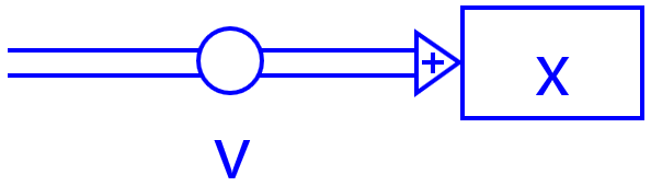
$$ v = dx/dt $$Difference equation:
$$\Delta x = v \cdot \Delta t $$Text-based model
\(\begin{array}{l} x = x + v \cdot dt\\ t = t + dt \end{array}\)Graphical model
Initial values (SI)
\(\begin{array}{l} v = 5\\ x = 0 \\ t = 0\\ dt = 0{.}1 \end{array}\)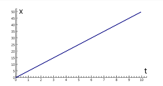
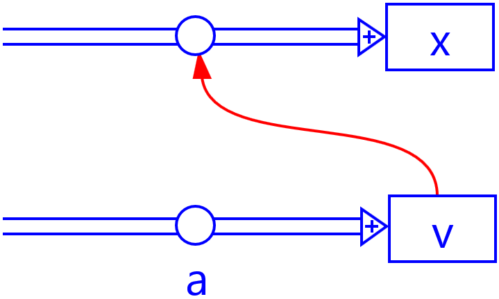
In this model, the velocity changes as a result of a constant acceleration.
The change of velocity is first calculated, after which the new velocity is used to calculate
the change of position.
With this model for instance, one can iteratively compute the motion of
the free fall.
Formulas in Binas:
$$ a = dv/ dt \quad v = dx/dt $$Difference equations:
$$\begin{array}{l} \Delta v = a \cdot \Delta t \\ \Delta x = v \cdot \Delta t \end{array}$$Text-based model
\(\begin{array}{l} v = v + a \cdot dt \\ x = x + v \cdot dt \\ t = t + dt \end{array}\)Graphical model
Initial values (SI)
\(\begin{array}{l} a = 5\\ v = 0\\ x = 0 \\t = 0 \\ dt = 0{.}1 \end{array}\)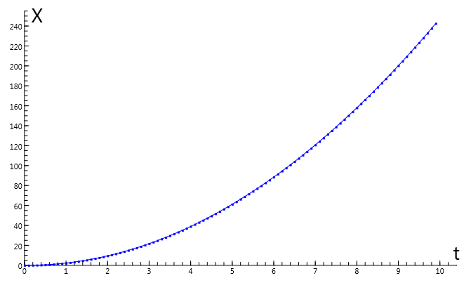
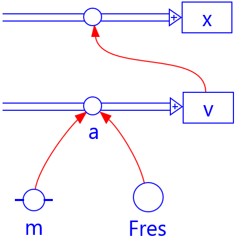
In this general dynaic model, Newton's second law of motion is recursively implemented
for some resultant force \(F_{\rm{res}}\), i.e. the sum of all forces, considered as vectors,
that are present in the given problem situation. The resultant force may depend on position
and/or velocity.
With this general model, realistic dynamic systems can be modelled with the
resultant force, the mass, and the initial values of the position and velocity as input.
Formulas in Binas:
$$\begin{array}{l} F_{\rm{res}} = m \cdot a \\ a = dv/ dt \quad v = dx/dt \end{array}$$Difference equations:
$$ \begin{array}{l} \Delta v = ({F_{\rm res}}/m) \cdot \Delta t \\ \Delta x = v \cdot \Delta t \end{array}$$Text-based model
\(\begin{array}{l} a = F_{\rm res}/m\\ v = v + a \cdot dt\\ x = x + v \cdot dt\\ t = t + dt \end{array}\)Graphical model
Initial values (SI)
\(\begin{array}{l} {F_{\rm res}} = 500\\ m = 650\\ v = 25\\ x = 0 \\ t = 0 \\ dt = 0{.}1 \end{array}\)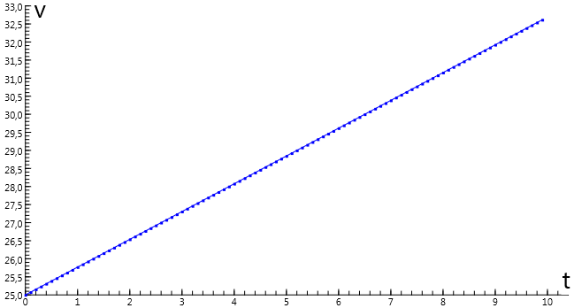
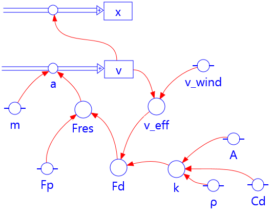
In this example of a dynamic model the bicyclist delivers a constant propulsive force \(F_{\rm p}\), but there is also a velocity dependent counteracting force \(F_{\rm d}\) as a consequence of drag (air restistance). The force is proportional to the square of the effective velocity of the bicyclist, i.e. the velocity corrected for head wind.
Formula in Binas:
$${F_{\rm{d}}} = \frac{1}{2} \rho \cdot {C_{\rm d}} \cdot A \cdot v^2 $$Difference equations:
$$\begin{array}{l} \Delta v = ({F_{\rm p}}/m -{F_{\rm d}}/m) \cdot \Delta t\\ \Delta x = v \cdot \Delta t \end{array}$$Text-based model
\(\begin{array}{l} v_{\rm eff}= v - v_{\rm wind} \\k= \frac{1}{2} \rho \cdot C_{\rm d} \cdot A\\ {F_{\rm d}} = k \cdot {v_{\rm eff}^2}\\ {F_{\rm {res}}} = {F_{\rm p}} - {F_{\rm d}}\\ a = {F_{\rm {res}}}/m\\ v = v + a \cdot dt\\ x = x + v \cdot dt\\ t = t + dt \end{array}\)Graphical model
Initial values (SI)
\(\begin{array}{l} {F_{\rm p}} = 40 \\ \rho=1{.}293\\ C_{\rm d}= 1.0\\A=0{.}55\\ m = 85\\ v_{\rm wind} = -7 \\ v = 0\\ x = 0 \\ t = 0\\ dt = 0.1 \end{array}\)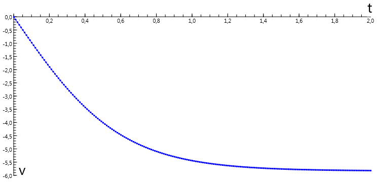
In this model, the vertical fall of an object with a large air resistance is modelled. An example is the shuttlecock used in the badminton game. The results obtained with the parameter values in the example below can be compared with a video analysis of experiments of the falling motion of a shuttlecock.5 The area A is calculated as the square of the maximum diameter of the shuttlecock.
Formulas in Binas:
$$\begin{array}{l} {F_{\rm d}} = \frac{1}{2} \rho \cdot {C_{\rm d}} \cdot A\ \cdot {v^2}\\ {F_{\rm g}} = m \cdot g \end{array}$$Difference equations:
$$\begin{array}{l} \Delta v = ( - g + F_{\rm d}/m )\cdot \Delta t \\ \Delta y = v \cdot \Delta t \end{array}$$Text-based model
\(\begin{array}{l} A= \frac{1}{4} \pi \cdot d^2\\ k = \frac{1}{2} \rho \cdot {C_{\rm d}} \cdot A\\ {F_{\rm d}} = k \cdot {v^2}\\ F_{\rm g} = m \cdot g \\ F_{\rm res} = - F_{\rm g} + F_{\rm d}\\ a = F_{\rm res} /m\\ v = v + a \cdot dt\\ y = y + v \cdot dt\\ t = t + dt \end{array}\)Graphical model
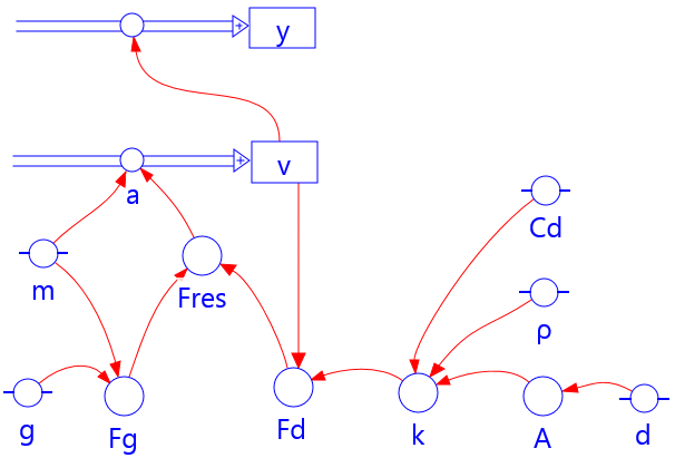
Initial values (SI)
\(\begin{array}{l} \rho = 1{.}293 \\ {C_{\rm d}} = 0{.}60\\ d= 0{.}057\\ m = 0{.}00328\\ g = 9{.}81\\ v = 0\\ y = 10 \\t = 0\\ dt = 0{.}01 \end{array}\)
In the parachute model the falling motion is modelled with a variable air resistance
via a 'If-Then' function. This function works as follows:
If [condition] Then [computation when the condition is satisfied]
Else [computation when the condition is satisfied] EndIf.
In this way the area A of the parachute, and herewith the air resistance,
become variable. The value of \(C_{\rm d}\) is kept constant, but the model can be adjusted
so that also this value changes.
Formulas in Binas:
$$\begin{array}{l} {F_{\rm d}} = \frac{1}{2} \rho \cdot {C_{\rm d}} \cdot A\;\\ {F_{\rm g}} = m \cdot g \end{array}$$Difference equations:
$$\begin{array}{l}\Delta v = ({F_{\rm g}}/m -{F_{\rm d}}/m) \cdot \Delta t \\ \Delta y = - v \cdot \Delta t \end{array}$$Text-based model
\(\begin{array}{l} \rm{If}\; y > 450 \\\quad {\rm Then}\; A = 0{.}8 \\ \quad {\rm Else}\; A = 42{.}6\\ \rm{EndIf}\\ k = {\textstyle{1 \over 2}} \rho \cdot {C_{\rm d}} \cdot A\\ {F_{\rm d}} = k \cdot {v^2}\\ F_{\rm g}= m \cdot g \\ F_{\rm res}= -F_{\rm g} +F_{\rm d}\\ a= F_{\rm res} / m \\ v = v + a \cdot dt\\ y = y + v \cdot dt\\ t = t + dt \end{array}\)Graphical model
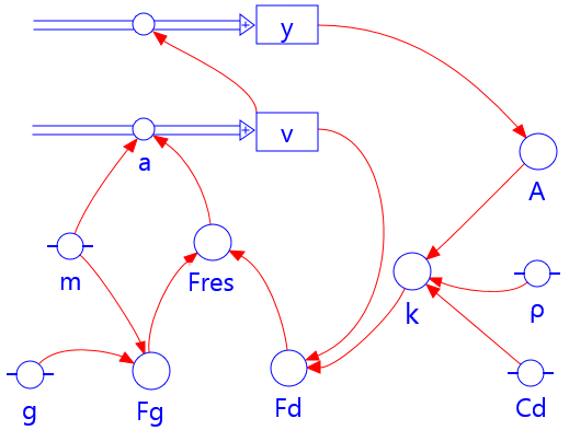
Initial values (SI)
\(\begin{array}{l} \rho = 1{.}293\\ {C_{\rm d}} = 0{.}69\\ m = 70\\ g = 9{.}81\\ v = 0\\ y = 1480 \\t = 0\\ dt = 0{.}05 \end{array}\)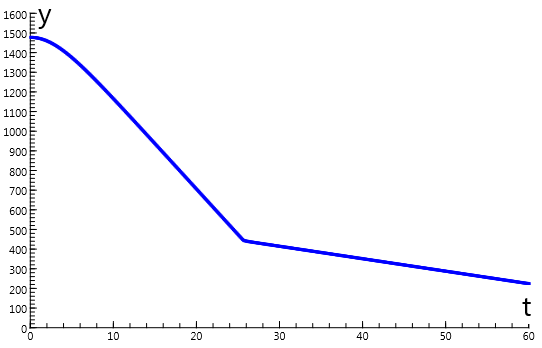
The ballistic trajectory model is an extension of the constant acceleration model to two spatial dimensions. The x- and y-coordinates of the velocity and position are calculated separately. The time-dependent speed of the bullet is also calculated.
Formula in Binas:
$${F_g} = m \cdot g$$Difference equations:
$$\begin{array}{l} \Delta {v_x}=0 \\ \Delta {v_y} = - g \cdot \Delta t \end{array}$$Text-based model
\(\begin{array}{l} v = \sqrt {v_x^2 + v_y^2} \\ {v_y} = {v_y} - g \cdot dt \\ x = x + {v_x} \cdot dt \\ y = y + {v_y} \cdot dt\\ t = t + dt \end{array}\)Graphical model
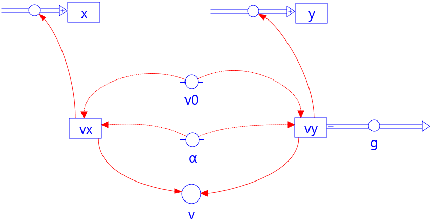
Initial values (SI)
\(\begin{array}{l} g = 9{.}81\\ {v_0} = 12\\ \alpha = 45\\ {v_y} = {v_0}\sin \alpha \\ {v_x} = {v_0}\cos \alpha \\ x = 0\\ y = 2 \\ t = 0\\ dt = 0{.}01 \end{array}\)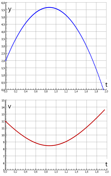
In the satellite model, the orbit is calculated of a light mass around a heavy mass \(M\). In this case, the mass of the satellite is not important and it is possible to calculate the gravitational acceleration due to the heavy mass $$ a_{\rm g} = \frac{{G \cdot M}}{r^2}$$ instead of the gravitational force \(F_{\rm g} \). The position and velocity are decomposed in the x- and y-directions. In principle, the orbit is elliptical, but depending on the initial values the orbit can also be circular (see the example).
Formula in Binas:
$${F_{\rm g}} = G \cdot \frac{{m \cdot M}}{{{r^2}}}$$Difference equations:
$$ \begin{array}{ll} {\Delta v_x} = a_x \cdot \Delta t & a_x = - {\displaystyle \frac{x}{r}}\cdot a_{\rm g}\\ \Delta x = v_x \cdot \Delta t & \\ {\Delta v_y} = a_y \cdot \Delta t & a_y = - {\displaystyle \frac{y}{r}}\cdot a_{\rm g}\\ \Delta y = v_y \cdot \Delta t & \end{array} $$The model is symmetric: there is no distinction between the x- and y-coordinate.
Text-based model
\(\begin{array}{l} r = \sqrt {{x^2} + {y^2}} \\ {a_{\rm g}} = \frac{{G \cdot M}}{{{r^2}}} \\ {a_x} = - \frac{x}{r}\cdot {a_{\rm g}} \\ {a_y} = - \frac{y}{r}\cdot {a_{\rm g}}\\ {v_x} = {v_x} + {a_x} \cdot dt \\ {v_y} = {v_y} + {a_y} \cdot dt\\ x = x + {v_x} \cdot dt \\ y = y + {v_y} \cdot dt\\ t = t + dt \end{array}\)Graphical model
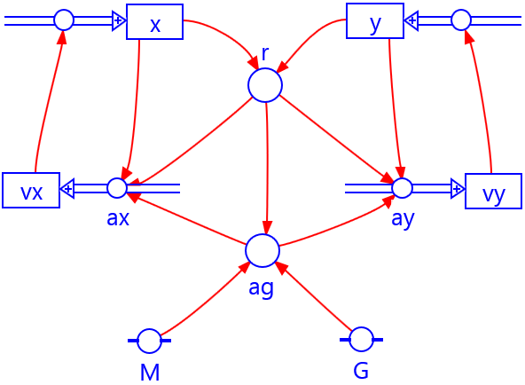
Initial values (SI)
\(\begin{array}{l} G = 6{.}67 \cdot {10^{ - 11}} \\ M = 5{.}97 \cdot {10^{24}}\\ {v_x} = 0 \\ {v_y} = 7248\, ({\rm circle})\\ {v_y} = 9100\, ({\rm ellipse})\\ x = 7{.}58 \cdot {10^6} \\ y = 0 \\t = 0 \\ dt = 1 \end{array}\)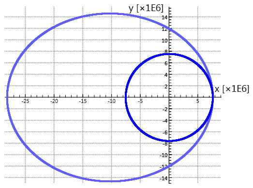
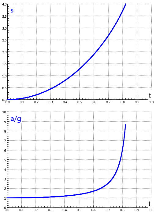
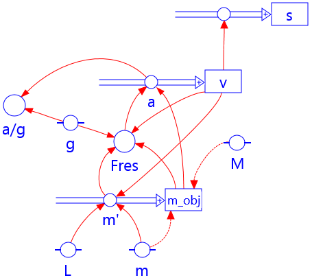
This model is about a falling mass model \( M\) on a chain of length \(L\) and
mass \( m\). The other end is connected to a fixed point \(y=0\).
In the initial situation the mass \(M\) is at the point \(y=0\) and the chain hangs
down in a loop to half the length.6
The mass that is going to fall is \(M\) plus half of the mass of the chain
\(m_{\rm obj} = M + \frac{1}{2}m \). During the falling motion this mass changes according to the formula
$$m_{\rm obj} = M + \frac{L-s}{2L} \cdot m $$ where \(s=-y\) denotes the displacement.
The change of mass with respect to time \(m'_{\rm obj}= dm_{\rm obj}/dt \) contributes to the resultant
force in the difference equation of this model.7
This leads to the remarkable conclusion that the acceleration \(F_{\rm res}/m_{\rm
obj}\) of the mass \(M\) is greater than the gravitational acceleration \(g\) (linked with free fall motion) because
\( m'_{\rm obj}< 0\). The effect is highly dependent on the mass ratio
\(\mu=m/M\). This can be verified by computing the model for a number of values of \( \mu \).
Formulas in Binas:
$$\begin{array}{l}{F_{\rm g}} = m \cdot g\\ F=dp/dt= m \cdot a + (dm/dt) \cdot v \end{array}$$Difference equations:
$$ \begin{array}{l} {\Delta m_{\rm obj}} = m'_{\rm obj} \cdot \Delta t \quad m'_{\rm obj}=-(m\cdot v)/{2L}\\ F_{\rm res} = m_{\rm obj}\cdot g - \frac{1}{2} m'_{\rm obj} \cdot v \\ {\Delta v} = (F_{\rm res}/m_{\rm obj}) \cdot \Delta t \\ \Delta s = v \cdot \Delta t \end{array} $$Text-based model
\(\begin{array}{l} m'= -(m \cdot v)/2L\\ m_{\rm obj}=m_{\rm obj} + m' \cdot dt\\ F_{\rm res} = m_{\rm obj}\cdot g - \frac{1}{2} m' \cdot v\\ a= F_{\rm res}/ m_{\rm obj}\\ v= v + a \cdot dt \\ s = s + v \cdot dt\\ t = t + dt \end{array}\)Graphical model
Initial values (SI)
\(\begin{array}{l} g = 9{.}81 \\ L=4 \\m = 0{.}75\\M = 0{.}125 \\ m_{\rm obj} = M+ \frac{1}{2}m\\ v = 0\\ s = 0 \\t = 0 \\ dt = 0{.}001 \end{array}\)