Examples of Convolutions
Definition and Calculation
The definition for the convolution \(G=F\star W\) of two discrete functions \(F\) and \(W\) is:
The recipe to calculate the convolution is:
- Mirror the function \(W\) in the origin to give function \(W^m[i,j]=W[-i,-j]\),
- then shift the weight function \(W^m\) to position \((k,l)\) in the image,
- pixelwise multiply the function and shifted weight function and
- sum all resulting values, this is the result of the convolution at point \((i,j)\).
Let’s do this for a simple example. Below you see a small image \(F\) and a weight function \(W\). Here we use the convention that when drawing weight functions (also called kernels) we assume it is defined over the infinite two dimensional domain, but we indicate only those values different from zero (note that points \((k,l)\) such that \(W[k,l]=0\) do not add to the convolution result, we simply can ignore those points).
In [1]: from scipy.ndimage import convolve;
In [2]: F = np.random.randint(0,10,(15,15)); print(F)
[[5 3 1 0 9 6 1 1 6 0 0 7 6 6 6]
[6 0 7 4 5 5 1 2 5 9 3 0 6 3 2]
[8 2 3 0 4 3 7 2 0 4 7 7 2 1 6]
[4 8 5 8 3 7 0 5 6 9 2 5 2 1 1]
[3 8 5 2 1 7 0 9 0 7 6 7 2 1 4]
[1 7 2 5 0 9 5 0 1 5 0 1 4 2 8]
[3 5 3 8 3 0 7 4 9 0 5 8 8 3 2]
[9 8 3 7 1 4 2 8 4 0 0 9 6 6 3]
[4 1 5 6 7 7 9 1 8 7 0 4 2 7 9]
[3 3 6 9 8 8 3 8 0 8 2 4 4 5 0]
[9 4 2 0 5 8 3 1 8 0 5 5 8 5 9]
[6 9 7 4 7 4 9 0 2 1 0 1 3 5 3]
[3 1 7 7 4 1 0 6 1 4 0 8 7 0 0]
[8 8 0 5 3 4 4 2 4 8 4 6 4 9 7]
[5 4 2 7 8 8 4 7 9 1 7 3 8 4 3]]
In [3]: W = np.ones((3,3))/9.0; print(W)
����������������������������������������������������������������������������������������������������������������������������������������������������������������������������������������������������������������������������������������������������������������������������������������������������������������������������������������������������������������������������������������������������������������������������������������������������������������������������������������������������������������[[ 0.11111111 0.11111111 0.11111111]
[ 0.11111111 0.11111111 0.11111111]
[ 0.11111111 0.11111111 0.11111111]]
In [4]: G = convolve(F,W); print(G)
��������������������������������������������������������������������������������������������������������������������������������������������������������������������������������������������������������������������������������������������������������������������������������������������������������������������������������������������������������������������������������������������������������������������������������������������������������������������������������������������������������������������������������������������������������������������������������������������������������������������������������������[[4 3 2 4 4 4 2 2 3 3 2 3 5 5 4]
[4 3 2 3 3 4 3 2 3 3 4 4 4 4 4]
[5 4 4 4 4 3 3 3 4 4 5 3 3 2 2]
[5 5 4 3 3 3 4 3 4 4 6 4 3 2 2]
[4 4 5 3 4 3 4 2 4 4 4 3 2 2 3]
[3 4 5 3 3 3 4 3 3 3 4 4 4 3 3]
[5 4 5 3 4 3 4 4 3 2 3 4 5 4 4]
[5 4 5 4 4 4 4 5 4 3 3 4 5 5 4]
[4 4 5 5 6 5 5 4 4 3 3 3 5 4 4]
[4 4 4 5 6 6 5 4 4 4 3 3 4 5 5]
[5 5 4 5 5 6 4 3 3 2 2 3 4 4 4]
[5 5 4 4 4 4 3 3 2 2 2 4 4 4 3]
[5 5 5 4 4 4 3 3 3 2 3 3 4 4 3]
[5 4 4 4 5 4 4 4 4 4 4 5 5 4 3]
[5 4 4 4 6 5 5 5 5 5 4 5 5 5 4]]
Read the documentation of the convolve function (it is in
scipy.ndimage) and make sure you understand its mode and
cval parameters. Note when working in IPython you can type ?
name where name is a function name, this will display the help
for that function.
In [5]: W2 = np.array([[1, 0, -1], [1, 0, -1], [1, 0, -1]]) / 3.0;

In [6]: print(W2)
[[ 0.33333333  0.         -0.33333333]
 [ 0.33333333  0.         -0.33333333]
 [ 0.33333333  0.         -0.33333333]]
What is the result of the convolution convolve(F,W2). Make the
calculation for 2 or 3 points in the image and take one of these on
the border of the image. Then compare your own calculation with
running the code.
Exercises A
Consider the one dimensional sampled function \(F\):
Calculate \(F\star W_1\) with:
\[W_1 = \pmatrix{1&\underline{1}&1}\]where the underline element denotes the origin (i.e. \(W[0]\)).
Calculate \(F\star W_2\) with:
\[W_2 = \pmatrix{1&\underline{0}&-1}\]
Properties
The convolution is both commutative, i.e. \(f\ast g=g\ast f\) and
associative, i.e. \((f\ast g)\ast h = f\ast(g\ast h)\). Note however
that the convolve function has neither of these properties. This
doesn’t imply that convolve does not implements the convolution
operator. It does but with some quirks due to the need for efficient
(fast) algorithms.
The commutative operator assumes that both operands are on equal
footing. In practice they are not. The first operand in \(f\ast w\), and
its implementation convolve(F,W) is the image \(f\) (discrete
F), most often very large, and the second operand is \(w\) (W)
is most often very much smaller. The convolve function takes an
image F and convolves it with W and returns the result. It
differs from the theory in the following aspects:
- the size of the result is set to be the size of the original image (that is a simplification because convolution with a \(3\times3\) kernel would theoreticall enlarge the image footprint—the pixels where it is different from zero—with one pixel along all sides).
- the border problem is solved in an adhoc way (read the explanation
of the
modeparamater) making the theoretical properties not true at the borders of the image.
Nevertheless we most often see in theory that the model of infinite images is used in image processing. Very seldomly people go into the trouble of modelling the finite size of the image domain.
For instance theory tells us that
but in practice:
In [7]: F = np.array([1,1,1]);
In [8]: print(convolve(F,F))
[3 3 3]
In [9]: print(convolve(F,F,mode='constant', cval=0))
��������[2 3 2]
Both wrong, but the second one less wrong then the first. Note that in
this simple example we see the two practical ‘shortcuts’ in action. We
can do better by embedding the original image F into a larger
array of zeros. Then the border effect are not influencial anymore.
In [10]: F0 = np.array([0,0,0,0,0,0,1,1,1,0,0,0,0,0,0]);
In [11]: print(convolve(F0,F))
[0 0 0 0 0 1 2 3 2 1 0 0 0 0 0]
In [12]: print(convolve(F0,F0))
��������������������������������[0 0 0 0 0 1 2 3 2 1 0 0 0 0 0]
Separable Convolution Kernels
We know that the \(5\times5\) uniform kernel is separable in two 1D convolution: one along the rows followed by a convolution along the columns:
In [13]: I = np.zeros((15, 15)); I[7, 7]=1;
In [14]: H = convolve(I, np.ones((1, 5))); print(H)
[[ 0. 0. 0. 0. 0. 0. 0. 0. 0. 0. 0. 0. 0. 0. 0.]
[ 0. 0. 0. 0. 0. 0. 0. 0. 0. 0. 0. 0. 0. 0. 0.]
[ 0. 0. 0. 0. 0. 0. 0. 0. 0. 0. 0. 0. 0. 0. 0.]
[ 0. 0. 0. 0. 0. 0. 0. 0. 0. 0. 0. 0. 0. 0. 0.]
[ 0. 0. 0. 0. 0. 0. 0. 0. 0. 0. 0. 0. 0. 0. 0.]
[ 0. 0. 0. 0. 0. 0. 0. 0. 0. 0. 0. 0. 0. 0. 0.]
[ 0. 0. 0. 0. 0. 0. 0. 0. 0. 0. 0. 0. 0. 0. 0.]
[ 0. 0. 0. 0. 0. 1. 1. 1. 1. 1. 0. 0. 0. 0. 0.]
[ 0. 0. 0. 0. 0. 0. 0. 0. 0. 0. 0. 0. 0. 0. 0.]
[ 0. 0. 0. 0. 0. 0. 0. 0. 0. 0. 0. 0. 0. 0. 0.]
[ 0. 0. 0. 0. 0. 0. 0. 0. 0. 0. 0. 0. 0. 0. 0.]
[ 0. 0. 0. 0. 0. 0. 0. 0. 0. 0. 0. 0. 0. 0. 0.]
[ 0. 0. 0. 0. 0. 0. 0. 0. 0. 0. 0. 0. 0. 0. 0.]
[ 0. 0. 0. 0. 0. 0. 0. 0. 0. 0. 0. 0. 0. 0. 0.]
[ 0. 0. 0. 0. 0. 0. 0. 0. 0. 0. 0. 0. 0. 0. 0.]]
In [15]: W = convolve(H, np.ones((5, 1))); print(W)
����������������������������������������������������������������������������������������������������������������������������������������������������������������������������������������������������������������������������������������������������������������������������������������������������������������������������������������������������������������������������������������������������������������������������������������������������������������������������������������������������������������������������������������������������������������������������������������������������������������������������������������������������������������������������������������������������������������������������������������������������������������������������������������������������������������������������������������������������������������������������������������������������������������������������������������������������������������������������������[[ 0. 0. 0. 0. 0. 0. 0. 0. 0. 0. 0. 0. 0. 0. 0.]
[ 0. 0. 0. 0. 0. 0. 0. 0. 0. 0. 0. 0. 0. 0. 0.]
[ 0. 0. 0. 0. 0. 0. 0. 0. 0. 0. 0. 0. 0. 0. 0.]
[ 0. 0. 0. 0. 0. 0. 0. 0. 0. 0. 0. 0. 0. 0. 0.]
[ 0. 0. 0. 0. 0. 0. 0. 0. 0. 0. 0. 0. 0. 0. 0.]
[ 0. 0. 0. 0. 0. 1. 1. 1. 1. 1. 0. 0. 0. 0. 0.]
[ 0. 0. 0. 0. 0. 1. 1. 1. 1. 1. 0. 0. 0. 0. 0.]
[ 0. 0. 0. 0. 0. 1. 1. 1. 1. 1. 0. 0. 0. 0. 0.]
[ 0. 0. 0. 0. 0. 1. 1. 1. 1. 1. 0. 0. 0. 0. 0.]
[ 0. 0. 0. 0. 0. 1. 1. 1. 1. 1. 0. 0. 0. 0. 0.]
[ 0. 0. 0. 0. 0. 0. 0. 0. 0. 0. 0. 0. 0. 0. 0.]
[ 0. 0. 0. 0. 0. 0. 0. 0. 0. 0. 0. 0. 0. 0. 0.]
[ 0. 0. 0. 0. 0. 0. 0. 0. 0. 0. 0. 0. 0. 0. 0.]
[ 0. 0. 0. 0. 0. 0. 0. 0. 0. 0. 0. 0. 0. 0. 0.]
[ 0. 0. 0. 0. 0. 0. 0. 0. 0. 0. 0. 0. 0. 0. 0.]]
Exercise B
The Sobel filter (in x-direction) is a filter that convolves an image with the kernel
\[\begin{split}\matvec{ccc}{ 1&0&-1\\ 2&0&-2\\ 1&0&-1}\end{split}\]This convolution is separable. What two kernels are being used in the separation?
To compare the speed of a separable filter or a true 2D filter you have to compare the time it takes to run a filter:
uniform_filter(f,s)versusconvolve(f,ones((s,s))/(s**2)). These two filters should give the same result but their timings are different. Run both filters on the same image for several values of s. Plot the graph of the run time versus the size of the filter. Compare the results, are they in accordance with what you expected?To time a piece of Python code you can use the
timefunction (from thetimepackage, so insert afrom time import timeline at the start of your code):startTime = time() # returns the actual time in seconds # here code to be timed elapsedTimeInSeconds = time()-startTime
Be aware that in case filters get very fast (say in the order of milliseconds) the accuracy when you time the execution of the filter once is very low, therefore in such cases you better time the execution time of the same filter repeated several times).
The Impulse Response Function
In the last piece of code we used a remarkable fact. An image completely zero except at one point is convolved with a kernel function and the kernel function itself is the result. This is true for any kernel. Let \(\Delta_{(a,b)}\) be the discrete function which is everywhere zero except at point \((a,b)\) where \(\Delta_{(a,b)}=1\), convolving this image with kernel \(W\) will result in an image where the kernel is shifted to position \((a,b)\):
This is a nice way to check whether a convolution does what it is meant to do.
In [16]: W = np.random.randint(1,10,(5,5)); print(W)
[[8 5 9 9 5]
[5 1 2 2 4]
[1 4 3 4 3]
[7 4 8 8 5]
[7 1 9 4 7]]
In [17]: F = convolve(I, W); print(F)
������������������������������������������������������������������[[ 0. 0. 0. 0. 0. 0. 0. 0. 0. 0. 0. 0. 0. 0. 0.]
[ 0. 0. 0. 0. 0. 0. 0. 0. 0. 0. 0. 0. 0. 0. 0.]
[ 0. 0. 0. 0. 0. 0. 0. 0. 0. 0. 0. 0. 0. 0. 0.]
[ 0. 0. 0. 0. 0. 0. 0. 0. 0. 0. 0. 0. 0. 0. 0.]
[ 0. 0. 0. 0. 0. 0. 0. 0. 0. 0. 0. 0. 0. 0. 0.]
[ 0. 0. 0. 0. 0. 8. 5. 9. 9. 5. 0. 0. 0. 0. 0.]
[ 0. 0. 0. 0. 0. 5. 1. 2. 2. 4. 0. 0. 0. 0. 0.]
[ 0. 0. 0. 0. 0. 1. 4. 3. 4. 3. 0. 0. 0. 0. 0.]
[ 0. 0. 0. 0. 0. 7. 4. 8. 8. 5. 0. 0. 0. 0. 0.]
[ 0. 0. 0. 0. 0. 7. 1. 9. 4. 7. 0. 0. 0. 0. 0.]
[ 0. 0. 0. 0. 0. 0. 0. 0. 0. 0. 0. 0. 0. 0. 0.]
[ 0. 0. 0. 0. 0. 0. 0. 0. 0. 0. 0. 0. 0. 0. 0.]
[ 0. 0. 0. 0. 0. 0. 0. 0. 0. 0. 0. 0. 0. 0. 0.]
[ 0. 0. 0. 0. 0. 0. 0. 0. 0. 0. 0. 0. 0. 0. 0.]
[ 0. 0. 0. 0. 0. 0. 0. 0. 0. 0. 0. 0. 0. 0. 0.]]
Exercises C
In these exercises the image I is the supposed to be the 15x15
image with all zeros except at the center where the value is 1.
The following functions from
scipy.ndimageare all convolutions. Calculate the impulse responses for:- laplace
- sobel
- prewitt
- gaussian_laplace
Some of these functions have parameters that result in different kernels being used.
Also run the filters on the cameraman image (or any other image of your liking). Comment on what you expect (or have read) the filter is supposed to do.
Another filter in the scipy.ndimage package is the maximum filter. The result of
maximum_filter(I,(5,5))andconvolve(I,ones((5,5)))are the same. Can we conclude that they are the same filter? Give an argumentation for your answer.
The Gaussian Convolution
Convolution with a Gaussian function can be done with the
gaussian_filter that is in the scipy.ndimage package. First we
start to see whether the impulse response function indeed looks like a
Gaussian function.
In [18]: from scipy.ndimage import gaussian_filter
In [19]: G1 = gaussian_filter(I, 1); print((100*(G1/G1.max())).astype(int))
[[ 0 0 0 0 0 0 0 0 0 0 0 0 0 0 0]
[ 0 0 0 0 0 0 0 0 0 0 0 0 0 0 0]
[ 0 0 0 0 0 0 0 0 0 0 0 0 0 0 0]
[ 0 0 0 0 0 0 0 0 0 0 0 0 0 0 0]
[ 0 0 0 0 0 0 0 1 0 0 0 0 0 0 0]
[ 0 0 0 0 0 1 8 13 8 1 0 0 0 0 0]
[ 0 0 0 0 0 8 36 60 36 8 0 0 0 0 0]
[ 0 0 0 0 1 13 60 100 60 13 1 0 0 0 0]
[ 0 0 0 0 0 8 36 60 36 8 0 0 0 0 0]
[ 0 0 0 0 0 1 8 13 8 1 0 0 0 0 0]
[ 0 0 0 0 0 0 0 1 0 0 0 0 0 0 0]
[ 0 0 0 0 0 0 0 0 0 0 0 0 0 0 0]
[ 0 0 0 0 0 0 0 0 0 0 0 0 0 0 0]
[ 0 0 0 0 0 0 0 0 0 0 0 0 0 0 0]
[ 0 0 0 0 0 0 0 0 0 0 0 0 0 0 0]]
In [20]: G2 = gaussian_filter(I, 2); print((100*(G2/G2.max())).astype(int))
����������������������������������������������������������������������������������������������������������������������������������������������������������������������������������������������������������������������������������������������������������������������������������������������������������������������������������������������������������������������������������������������������������������������������������������������������������������������������������������������������������������������������������������������������������������������������������������������������������������������������������������������������������������������������������������������������������������������������������������������������������������������������������������������������������������������������������������������������������������������������������������������������������������������������������������������������������������������������������[[ 0 0 0 0 0 0 0 0 0 0 0 0 0 0 0]
[ 0 0 0 0 0 0 0 1 0 0 0 0 0 0 0]
[ 0 0 0 0 1 2 3 4 3 2 1 0 0 0 0]
[ 0 0 0 1 4 8 11 13 11 8 4 1 0 0 0]
[ 0 0 1 4 10 19 28 32 28 19 10 4 1 0 0]
[ 0 0 2 8 19 36 53 60 53 36 19 8 2 0 0]
[ 0 0 3 11 28 53 77 88 77 53 28 11 3 0 0]
[ 0 1 4 13 32 60 88 100 88 60 32 13 4 1 0]
[ 0 0 3 11 28 53 77 88 77 53 28 11 3 0 0]
[ 0 0 2 8 19 36 53 60 53 36 19 8 2 0 0]
[ 0 0 1 4 10 19 28 32 28 19 10 4 1 0 0]
[ 0 0 0 1 4 8 11 13 11 8 4 1 0 0 0]
[ 0 0 0 0 1 2 3 4 3 2 1 0 0 0 0]
[ 0 0 0 0 0 0 0 1 0 0 0 0 0 0 0]
[ 0 0 0 0 0 0 0 0 0 0 0 0 0 0 0]]
In [21]: G3 = gaussian_filter(I, 3); print((100*(G3/G3.max())).astype(int))
��������������������������������������������������������������������������������������������������������������������������������������������������������������������������������������������������������������������������������������������������������������������������������������������������������������������������������������������������������������������������������������������������������������������������������������������������������������������������������������������������������������������������������������������������������������������������������������������������������������������������������������������������������������������������������������������������������������������������������������������������������������������������������������������������������������������������������������������������������������������������������������������������������������������������������������������������������������������������������������������������������������������������������������������������������������������������������������������������������������������������������������������������������������������������������������������������������������������������������������������������������������������������������������������������������������������������������������������������������������������������������������������������������������������������������������������������������������������������������������������������������������������������������������������������������������������������������������������������������������������������������������������������������������������������������������������������������������������������������������������������������������������������������������������������������������������������������������������������������������������������������������������������������������������������������������������������������������������[[ 0 1 2 3 5 7 8 9 8 7 5 3 2 1 0]
[ 1 2 3 6 8 11 13 14 13 11 8 6 3 2 1]
[ 2 3 6 10 15 20 23 25 23 20 15 10 6 3 2]
[ 3 6 10 17 25 33 39 41 39 33 25 17 10 6 3]
[ 5 8 15 25 36 48 57 60 57 48 36 25 15 8 5]
[ 7 11 20 33 48 64 75 80 75 64 48 33 20 11 7]
[ 8 13 23 39 57 75 89 94 89 75 57 39 23 13 8]
[ 9 14 25 41 60 80 94 100 94 80 60 41 25 14 9]
[ 8 13 23 39 57 75 89 94 89 75 57 39 23 13 8]
[ 7 11 20 33 48 64 75 80 75 64 48 33 20 11 7]
[ 5 8 15 25 36 48 57 60 57 48 36 25 15 8 5]
[ 3 6 10 17 25 33 39 41 39 33 25 17 10 6 3]
[ 2 3 6 10 15 20 23 25 23 20 15 10 6 3 2]
[ 1 2 3 6 8 11 13 14 13 11 8 6 3 2 1]
[ 0 1 2 3 5 7 8 9 8 7 5 3 2 1 0]]
A 3D plot of the G1, G2 and G3 discrete kernel functions
are shown in the figure below.
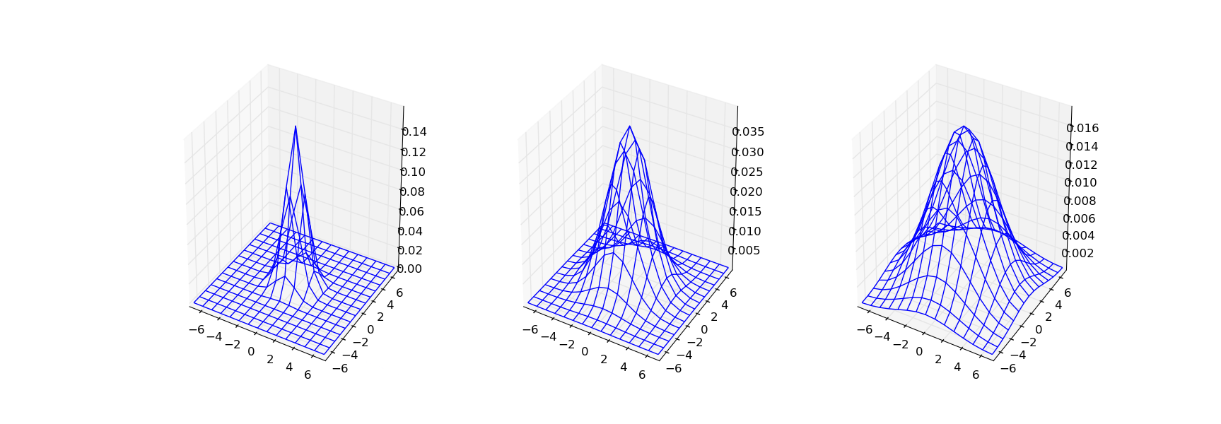
Gaussian Kernels. From left to right the Gaussian functions with s=1, s=2 and s=3 respectively.
Exercises D
- Compare the Gaussian filter with the uniform filter (use
functions
gaussian_filteranduniform_filter) using different sizes of the filter (the sigma parameter for the gaussian filter and the size parameter for the uniform filter). Subjectively determine what you think what the relation is between the size and sigma to have similar smoothing effect for both filters. - Run both filters on the cameraman image. Compare the results.
- Build a scale-space
F[i,j,k]where i and j are the spatial indices in a 3D array and k is the index of the scale axis. Use a logarithmic sampling of the scale axis \(s_k = \alpha^k s_0\). For the original image you may assume \(s_0=0.5\). Appropriate values for \(\alpha\) are around 1.5.