6.3.5. Extended Features in Logistic Regression
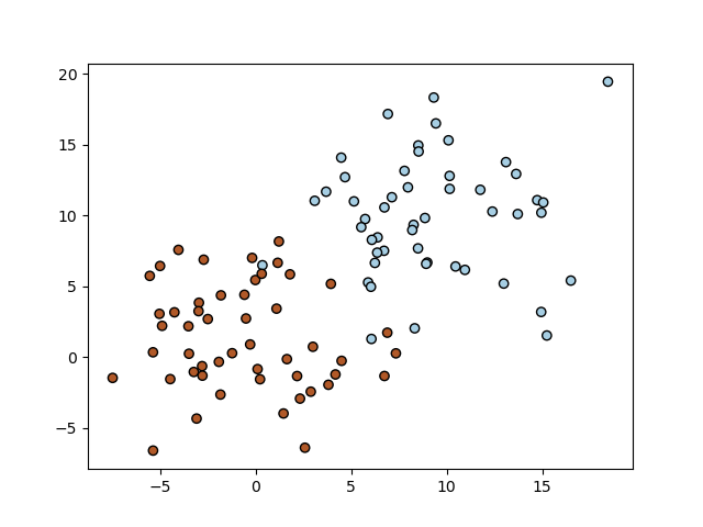
A logistic regression classifier in basic form finds a (hyper) plane in feature space that best separates the two classes. Consider the data shown in the figure below.
In [1]: from matplotlib.pylab import *

In [2]: m = 100

In [3]: X0 = 4*randn(m//2, 2) + (9, 9)

In [4]: y0 = zeros((m//2))

In [5]: X1 = 4*randn(m//2, 2) + (1, 1)

In [6]: y1 = ones((m//2))

In [7]: X = vstack((X0, X1))

In [8]: y = hstack((y0, y1))

In [9]: print(X0.shape, X1.shape, X.shape)
(50, 2) (50, 2) (100, 2)

In [10]: scatter(X[:,0], X[:,1], c=y, edgecolors='k', cmap=cm.Paired);

In [11]: show()
We will use a logistic regression classifier from sklearn. We set C=10000 to effectively switch off regularization.
In [12]: from sklearn.linear_model import LogisticRegression

In [13]: logregr = LogisticRegression(C=10000, fit_intercept=True)

In [14]: logregr.fit(X,y)
Out[14]: LogisticRegression(C=10000)

In [15]: xmin = X[:,0].min() - 0.5

In [16]: xmax = X[:,0].max() + 0.5

In [17]: ymin = X[:,1].min() - 0.5

In [18]: ymax = X[:,1].max() + 0.5

In [19]: mx, my = meshgrid( arange(xmin, xmax, 0.1),
   ....:                    arange(ymin, ymax, 0.1) )
   ....:

In [20]: Z = logregr.predict(c_[mx.ravel(), my.ravel()])

In [21]: Z = Z.reshape(mx.shape)

In [22]: pcolormesh(mx, my, Z, cmap=cm.Paired);

In [23]: scatter(X[:,0], X[:,1], c=y, edgecolors='k', cmap=cm.Paired);

In [24]: show()
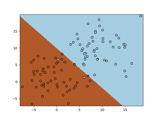
The figure above shows a well-known toy problem for logistic regression. The two classes are nicely linear seperable (with the exception of a few ‘outliers’). But now consider the classical XOR problem (well, we have added some noise to it…)
In [25]: from matplotlib.pylab import *

In [26]: m = 100

In [27]: X0 = 1.5*randn(m//2, 2) + (9, 9)

In [28]: y0 = zeros((m//2))

In [29]: X1 = 1.5*randn(m//2, 2) + (1, 1)

In [30]: y1 = zeros((m//2))

In [31]: X = vstack((X0, X1))

In [32]: y = hstack((y0, y1))

In [33]: X0 = 1.5*randn(m//2, 2) + (1, 9)

In [34]: y0 = ones((m//2))

In [35]: X1 = 1.5*randn(m//2, 2) + (9, 1)

In [36]: y1 = ones((m//2))

In [37]: X = vstack((X,X0,X1))

In [38]: y = hstack((y,y0,y1))

In [39]: scatter(X[:,0], X[:,1], c=y, edgecolors='k', cmap=cm.Paired);

In [40]: show()
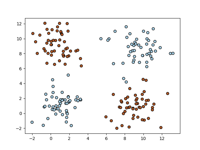
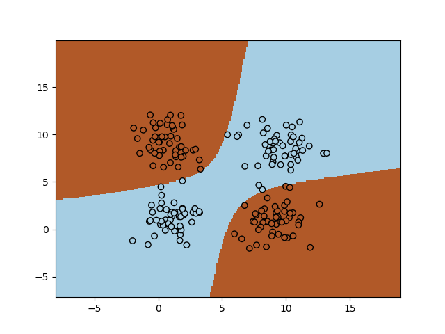
Evidently this is not a linearly seperable classification dataset. We can however add non linear (monomial) features to our dataset. Instead of only \(x_1\) and \(x_2\) we add \(x_1^2\), \(x_1 x_2\) and \(x_2^2\) (note that the bias is added automagically by sklearn.
In [41]: Xe = append(X,(X[:,0]**2)[:,newaxis],axis=1)

In [42]: Xe = append(Xe,(X[:,1]**2)[:,newaxis],axis=1)

In [43]: Xe = append(Xe,(X[:,0]*X[:,1])[:,newaxis],axis=1)

In [44]: logregr.fit(Xe,y)
Out[44]: LogisticRegression(C=10000)

In [45]: mxr = mx.ravel()

In [46]: myr = my.ravel()

In [47]: Z = logregr.predict(c_[mxr, myr, mxr**2, myr**2, mxr*myr])

In [48]: Z = Z.reshape(mx.shape)

In [49]: pcolormesh(mx, my, Z, cmap=cm.Paired);

In [50]: scatter(X[:,0], X[:,1], c=y, edgecolors='k', cmap=cm.Paired);

In [51]: show()