6.3.1. Logistic Regression Model
We start with a simple two class problem \(Y=0\) or \(Y=1\). The logistic regression classifier assumes that a hyperplane separates the two classes in feature space. In two dimensional feature space the hyperplane is a straight line, feature vectors on one side of the plane belong to the \(Y=0\) class, vectors on the other side belong to the \(Y=1\) class.
The a posteriori probability \(\P(Y=1\given \v X=\v x)\) is modelled with the hypothesis function \(h_{\v\theta}(\v x)\)
where \(\tilde{\v x} = (1\; \v x)\T\) is the feature vector \(\v x\) is augmented with a bias term. Note that the parameter vector \(\v\theta\) thus is a \(n+1\) dimensional vector.
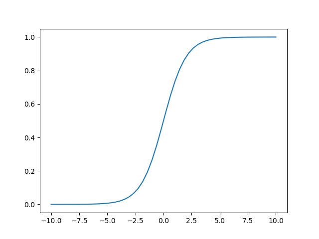
The function \(g\) is the sigmoid or logistic function and is defined as:
Plotting this function show that \(g(v)\) is in the range from \(0\) to \(1\) (what is to be expected for a probability of course).
Note that for a 2D (nD) feature space:
\(\v\theta\T\tilde{\v x} = 0\) defines a line (hyperplane) in feature space.
This line (hyperplane) is called the decision boundary, points \(\v x\) where \(h_{\v\theta}(\v x)>0.5\) are classified as \(y=1\), whereas points where \(h_{\v\theta}(\v x)<0.5\) are classified as \(y=0\).
On this line (hyperplane) we have \(h_{\v\theta}(\v x)=0.5\).
On lines (hyperplanes) parallel to the above line (hyperplane) the hypothesis value is constant.
Training a logistic regression classifier thus amounts to learning the optimal parameter vector \(\v\theta\) given a set of training examples \((\v x\ls i, y\ls i)\) for \(i=1,\ldots,m\). In the next section we will describe this learning process as a maximum likelihood estimator for \(\v\theta\).