6.4. Neural Networks
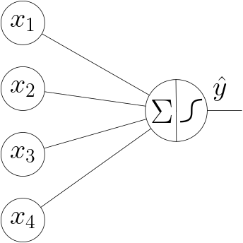
Fig. 6.4.1 Logistic Regression Unit. The bias value is not shown in this graph.
From a technical point of view a neural network is a collection of interconnected logistic regression units. One logistic regression unit takes in \(n\) input values, calculates a linear combination of those values using the ‘weights’ (parameters), adds a bias value and passes the resulting sum through a non-linear activation function. The resulting value (in case classification is the goal) approximates the a posteriori probability of the class \(y=1\) given the \(n\) feature values. Symbolically this is depicted in Fig. 6.4.1.
The input values \(x_1, \ldots,x_4\) are each multiplied with associated weight (parameter) \(\theta_i\), summed (and a bias weight \(\theta_0\) is added) and then fed through the activation function. The result is the value \(\hat y\) associated with that one output node in the graph.
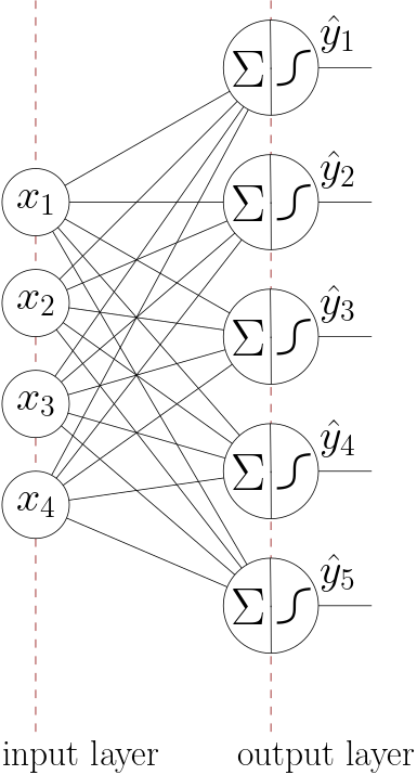
Fig. 6.4.2 Logistic Regression Units in parallel, working on the same input data.
To build a neural network we start by extendig this was logistic regression unit to \(m\) units where each of those units is fed with the same \(n\) input values. If we have \(m\) of those logistic regression units working in parallel on the same input values we end up with something like is depicted in Fig. 6.4.2.
From here on we can go on adding layers of nodes going from left to right. Adding two more layers to our example network ending in just one output node we end up with a network as shown in Fig. 6.4.3.
In the context of neural networks one logistic regression unit is called a neuron. Read the next section to learn that neural networks were indeed inspired by comparison with the brain where neurons are the basic information processing building blocks.
In a neural network we always have an input layer and an output layes. The number of nodes (values) in the input layer equals the number of feature values. The number of nodes in the output layer depends on the use of the neural network. For boolean classification we most often will have one node, whereas for a \(k\) classes classification task we often have \(k\) output nodes, one for each class.
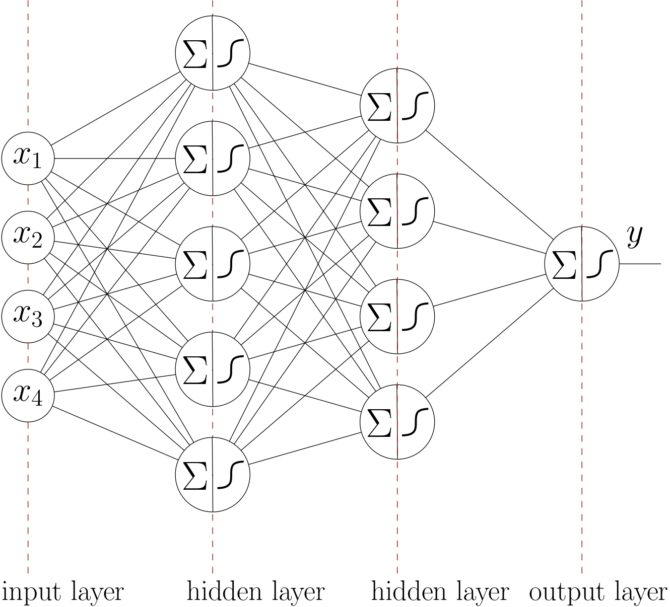
Fig. 6.4.3 Fully Connected Neural Network with 4 layers, 4 nodes in input layer and 1 node in the output layer.
The layers inbetween the input and output layers are called the hidden layers. Again note that the bias values can be used for all (logistic regression) nodes but are not shown in the graph.
As may be clear from this last network graph, the complexity becomes large and in a detailed description we need to keep track of all the nodes in all layers and all the weights involved. We will do in both the more classical way that closely resembles the graph in Fig. 6.4.3 and in a more modern formalism.
Learning the weights in a network with several layers needs a technique called back propagation. Remember that learning the parameters of the simple logistic regression (in Fig. 6.4.1) requires comparing the error (loss) between the desired output (the target value) and the value that is calculated by the hypothesis function. For the hidden layers in a neural network there is no target value available of course. Back propagation learning is really nothing else than using the chain rule of differentiation in a systematic way.
Important questions to be answered when using a neural network in practice are:
How many layers do i need for optimal performace and
how many nodes in each layer?
The first question has a surprising answer: only three layers are enough (i.e. only one hidden layer). Only one hidden layer can be proven to result in an hypothesis function that can approximate any functional relation between input values and output value.
There is a big catch there. The number of nodes needed in the hidden layer might become unpractically high. And furthermore such an ‘optimal’ network proves to be hard to learn using back propagation, the risk of overfitting is high.
Modern deep learning research has shown that very deep networkds (i.e. with a lot of layers in the order of hundreds) are indeed slow learners but with the best possible results.
To this day deciding on the number of layers and the number of nodes in a layer is more of an art than a science. Experimentation is key in this area.
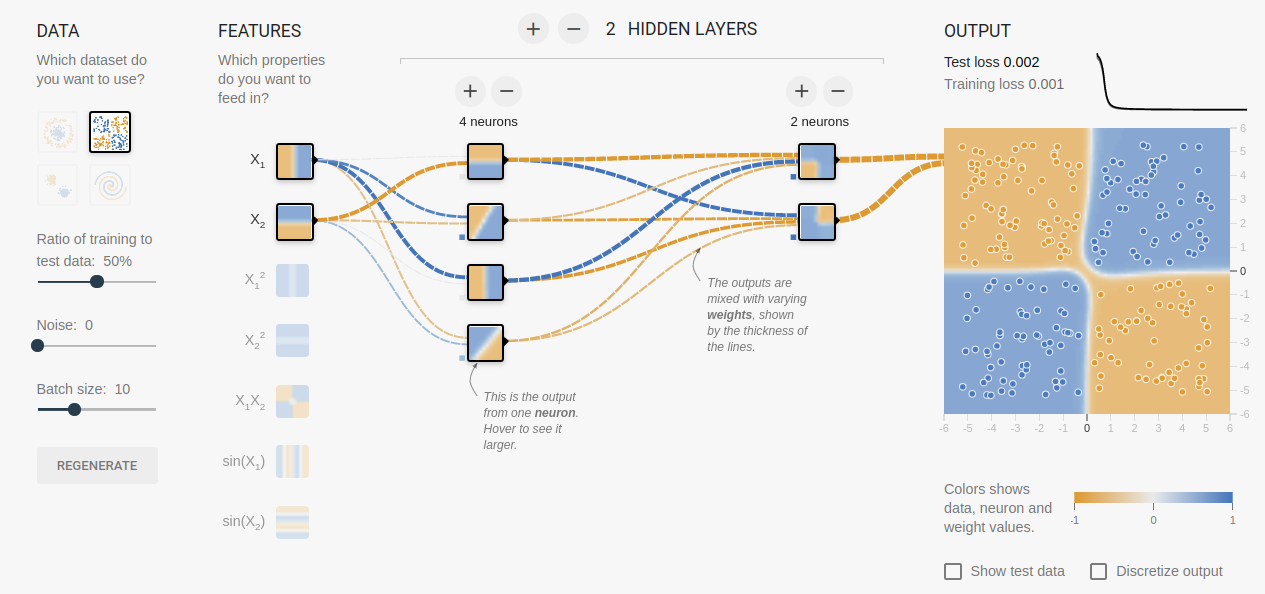
Fig. 6.4.4 Neural Network Playground (using the Tensor Flow deep learning framework). Shown is a network with two hidden layers solving the XOR problem.
To get some intuitive understanding of what a neural network is doing i urge you to play with a neural network at the TensorFlow playground (see Fig. 6.4.4 for a screenshot), an online demonstration that works on a two dimensional input vector \((x_1\;x_2)\T\) (and possibly some augmented features) with variable number of hidden layers and number of nodes in the hidden layers.