6.4.3. A Modern View On Neural Networks
In the more modern view on neural networks we will use graphs where the data is represented as the arrows in the graph and the nodes indicate the processing blocks.
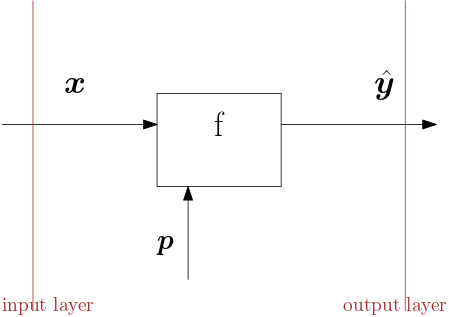
Fig. 6.4.10 One processing block or node in a neural network. A block or node represents the processing done going from one layer to the next.
The flow from input vector \(\v x\) to output vector \(y\) is represented in Fig. 6.4.10. The parameters that determine the processing are indicated with a vector \(\v p\) (later on we will use parameter matrices as well). Symbolically we can write:
When we cascade these blocks to form a network of fully connected processing nodes we get something like (assuming 3 processing nodes) depicted in Fig. 6.4.11.
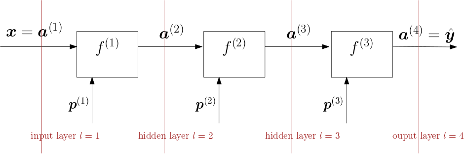
Fig. 6.4.11 Cascade of three processing blocks forming a fully connected neural network.
The input \(\v x\) - output \(\hat{\v y}\) relation for this network is:
where we use \(\hat{\v y}\) as the output of the network to indicate that it is an estimation of some desired target value \(\v y\).
When learning all the parameters in the network (in our case these are \(\v p\ls1\), \(\v p\ls2\) and \(\v p\ls3\)) in a supervised learning setting we calculate the loss \(\ell\) (cost) in comparing the output \(\hat{\v y}\) given input \(\v x\) with the known target value \(\v y\).
Extending the cascade (graph) with the loss calculation we have:
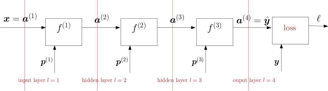
Fig. 6.4.12 Cascade of three processing blocks with loss calculation.
We sketch the graph for the loss calculation for one learning example \((\v x, \v y)\). For all values in the learning set (of for a subset of the learing set: a batch) the total loss is simply the sum of the individual losses.
Given the loss function, for instance the quadratic loss function:
The learning procedure tries to minimize the loss function using a gradient descent procedure. I.e. for all \(i=1,2,3\) it iterates steps:
Note that \(\ell\) is dependent on \(\hat{\v y}\) and thus dependent on all \(\v p\ls i\). In case we calculate the loss for the entire learning set or for a batch of examples the gradient is simply the sum of the gradients for the individual examples. Therefore we look at one example only in this introduction. In subsequent sections we will use larger batches of examples.
Also note that for differentiable functions \(f\ls i\) equations Eq.6.4.1 and Eq.6.4.2 show that the gradient can be calculated analytically and will require as many uses of the chain rule of differentiations as there are blocks in the cascade.
To guide us in our calculation of the gradients of the loss function with respect to the parameters in our network we will do it block by block starting at the output and working our way towards the input.
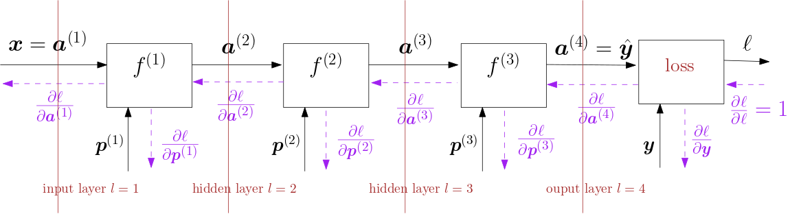
Fig. 6.4.13 Forward and backward pass.
In Fig. 6.4.13 the neural network with 4 layers (i.e. 3 processing blocks) and the loss block is sketched again but this time with backward arrows we also indicate the flow to calculate the derivatives of the loss function with respect to intermediate values in the network (including the parameters). For each block given the derivative of the loss with respect to its output we can calculate the derivative of the loss with respect to its inputs (including the parameters). That derivative requires only knowledge of that particular block. It is the chain rule that will tie all these derivatives together.
In a fully connected neural network each of the processing blocks \(f\ls i\) in the graphs above can be decomposed in steps as depicted in Fig. 6.4.14.
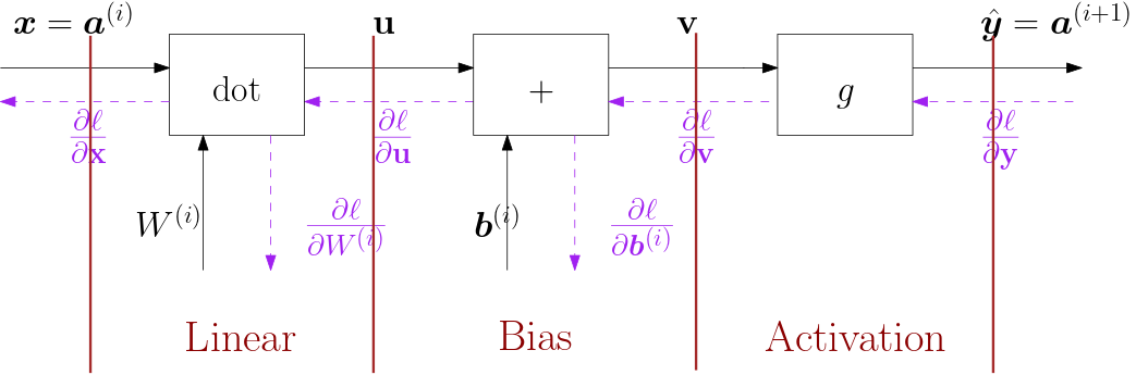
Fig. 6.4.14 One block(node) in a fully connected neural network.
Note that the parameter vector \(\v p\ls i\) is now split into the parameter matrix \(W\ls i\) and bias vector \(\v b\ls i\). In subsequent sections we will look at these blocks individually and then finally do it for an entire network (i.e. chain of processing blocks).
In order to appreciate the rest of this section (and chapter) you better refresh your understanding of the chain rule reading the math chapter on the chain rule in differentiation.