6.4.3.4. Loss Function

\(\newcommand{\in}{\text{in}}\) \(\newcommand{\out}{\text{out}}\) \(\newcommand{\prt}{\partial}\)

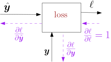
Fig. 6.4.18 Loss Function.

In this section we only consider the derivations for the \(L_2\) loss, i.e. the quadratic loss function:

\[\ell = \ell(\hat{\v y}, \v y) = \half \|\hat{\v y} - \v y\|^2\]

where \(\v y\) is the target value. Note that \(\hat{\v y}\) is the output of the entire neural network. In our loss function we have not incorporated any regularization term.

Here we have:

\[\pfrac{\ell}{\hat{\v y}} = \hat{\v y} - \v y\]

We see that is the error, i.e. the difference between what the network calculates for output (\(\hat{\v y}\)) and what it should be according to our learning set \(\v y\), that starts of the chain of backpropagation steps through all the layers from the front all the way backwards to the input.

Vectoring the loss function and derivate we get the cost for the entire batch as the sum of the individual losses.

\[J = \frac{1}{m} \sum_{i=1}^m \ell(\hat{\v y}\ls i, \v y\ls i) = \frac{1}{2m} \|\hat{Y} - Y\|_F^2\]

where \(\|\cdot\|_F\) is the Frobenius norm of a matrix (sum of all squared elements), \(\hat{Y}\) is the matrix of all outputs of the neural net (as rows in the matrix), and \(Y\) is the matrix of all target vectors as rows. Now the derivative becomes:

\[\pfrac{\ell}{\hat{Y}} = \frac{1}{m}(\hat{Y} - Y)\]