6.4.2. The Classical View on Neural Networks

In the classical view on neural networks graphs are used as well as in the modern view. In the classical graphs each node represents both a function as well as the value that it the outcome of that function., the edges in the graph indicate both the flow of values as well as the ‘connection strengths’ (the weight values).

A two layer network with one output node is the same as a logistic regression unit. The input layer contains \(n\) values (in the input nodes the values are not processed). In the node in the second layer we first calculate a weighted sum of the input values \(a_i\) and add a bias term to it

\[z = \theta_0 + \theta_1 a_1 + \cdots + \theta_n a_n = \v\theta\T\hv a\]

where \(\v a\) is the vector \((a_1\cdots a_n)\T\) and \(\hv a\) is the augmented vector \((1 \; a_1\cdots a_n)\T\). The extra element equal to 1 is added to ‘pick up’ the bias term \(\theta_0\). The final value is

\[a_{\text{out}} = g(z)\]

where \(g\) is the activation function.. For now think of the logistic function as it is also used in logistic regression.

Elementwise function application

The notation \(f(\v x)\) is read as applying a function that maps a vector \(\v x\) and returns a scalar. Essentially \(f(\v x)\) is short hand notation for

\[f(\v x) = f(x_1,\ldots,x_n)\]

In machine learning we often find the need to apply a scalar function to each of the elements in a vector (just like Numpy applies a function to all elements in an array). For this special case we will write \(f\aew(\v x)\):

\[\begin{split}f\aew(\v x) = \begin{pmatrix} f(x_1)\\ \vdots\\ f(x_n)\end{pmatrix}\end{split}\]

To get an entire layer in a nearal network we feed our input vector \(\hv a\) not in one logistic regression node but in \(m\) nodes. Each of those nodes is characterized with its own parameter vector \(\v\theta_j\) for \(j=1,\ldots,m\). Combining these into a weight matrix \(\Theta\)

\[\begin{split}\Theta = \begin{pmatrix} \v\theta_1\T \\ \v\theta_2\T \\ \vdots\\ \v \theta_m\T \end{pmatrix}\end{split}\]

The \(m\) outputs then are combined into one vector \({\v a}_\text{out}\). Given an input \({\hv a}_\text{in}\) we have:

\[\begin{split}\v z_\text{out} &= \Theta \hv a_\text{in}\\ \v a_\text{out} &= g\aew(\v z_\text{out})\end{split}\]

Carefully note that whereas the input is augmented (with the 1 element) the output is not augmented.

Now we can build a complete network with these layers of ‘logistic regression units’.

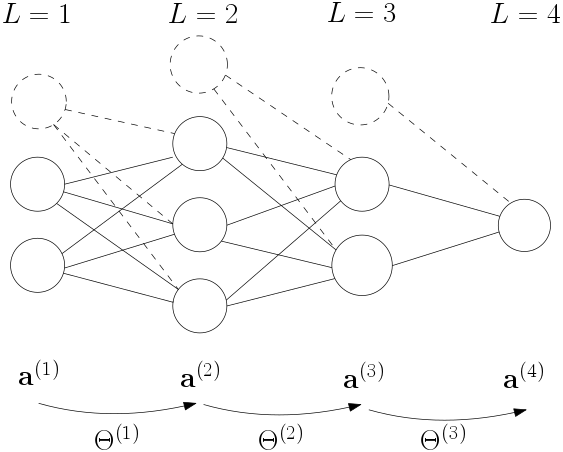
Fig. 6.4.9 A 4 layer neural network. The number of nodes in each of the layers is 2,3,2,1. The ‘bias nodes’ (dashed) are not counted. There are three weight matrices in this network \(\Theta\ls 1\), \(\Theta\ls 2\) and \(\Theta\ls 3\).

Note that in the classical view this is called a 4 layer network as the input nodes are called a layer as well (although nothing is calculated in that ‘layer’). A \(L\)-layer network is thus characterized with \(L-1\) weight matrices.

The values in the nodes in one layer are called the activation of that layer and we will write the activation in layer \(l\) as \(\v a\ls l\). We start numbering at 1 so \(\v a\ls 1\) is the input \(\v x\) to our network. Going from layer 1 to layer 2 we have:

\[\begin{split}\v z\ls 2 &= \Theta\ls 1 \hv a\ls 1 \\ \v a\ls 2 &= g\aew(\v z\ls 2)\end{split}\]

In general going from layer \(l\) to layer \(l+1\) we have:

\[\begin{split}\v z\ls {l+1} &= \Theta\ls l \hv a\ls l \\ \v a\ls {l+1} &= g\aew(\v z\ls {l+1})\end{split}\]

The final output of the network is \(\v a\ls L\). Formally we write

\[h_\v\Theta(\v x) = \v a\ls L\]

where the \(\v\Theta\) is used to indicate all weight matrices in the network, \(\v\Theta =\{\Theta\ls 1,\cdots\Theta\ls{L-1}\}\). Note that the above expression is sloppy math, the \(\v x\) in the left hand side is nowhere to be found on the right hand side. But evidently \(\v a\ls L\) depends ultimately on \(\v x = \v a\ls 1\).

Finding all the parameters in a neural network boils down to finding all weight matrices in the network. Assuming a mean squared error loss over a learning set of tuples \((\v x\ls i, \v y\ls i)\) for \(i=1,\ldots,m\), we have the following loss (cost) to be minimized:

\[J(\v\Theta) = \frac{1}{m} \sum_{i=1}^{m} \| h_\v\Theta(\v x\ls i) - \v y\ls i \|^2\]

We have left out a possible regularization term. Also note that the cross entropy error measure as used in logistic regression can be used here as well,

The minimization of the cost (or loss) function is the same as for all other minimization procedures that we have encountered before: gradient descent:

\[\forall l: \quad \Theta\ls l := \Theta\ls l - \alpha \frac{\partial J(\v\Theta)}{\partial\Theta\ls l}\]

In these lecture notes you will not find the expressions for the cost gradients (in this form). Instead we will first rewrite the neural network into the computational graph formalism and do the backpropagation in that formalism. The reason that we go that route is twofold. First the derivations are easier (IMHO). Secondly and more importantly the ‘language’ used is the one from the modern view on neural networks paving the way for a somewhat easier understanding of deep learning methodologies.