8.2.2. Lab week 2 DSP instrumentation

The purpose of this lab is to get some elementary experience with * analog signals in the time domain and visualisation of these signals using an oscilloscope. * Plotting a Bode diagram for amplitude and phase characteristics. * See the behavior of low pass and high pass filters.

During these lab we use some materials of the physics department. Write a short labreport of the experiments below and upload it into blackboard.

8.2.2.1. Assignment 1.

Connect the functiongenerator to the oscilloscope by using 2 mm wires and a BNC to 2mm connector. Use a sine wave output of about 1 kHz.

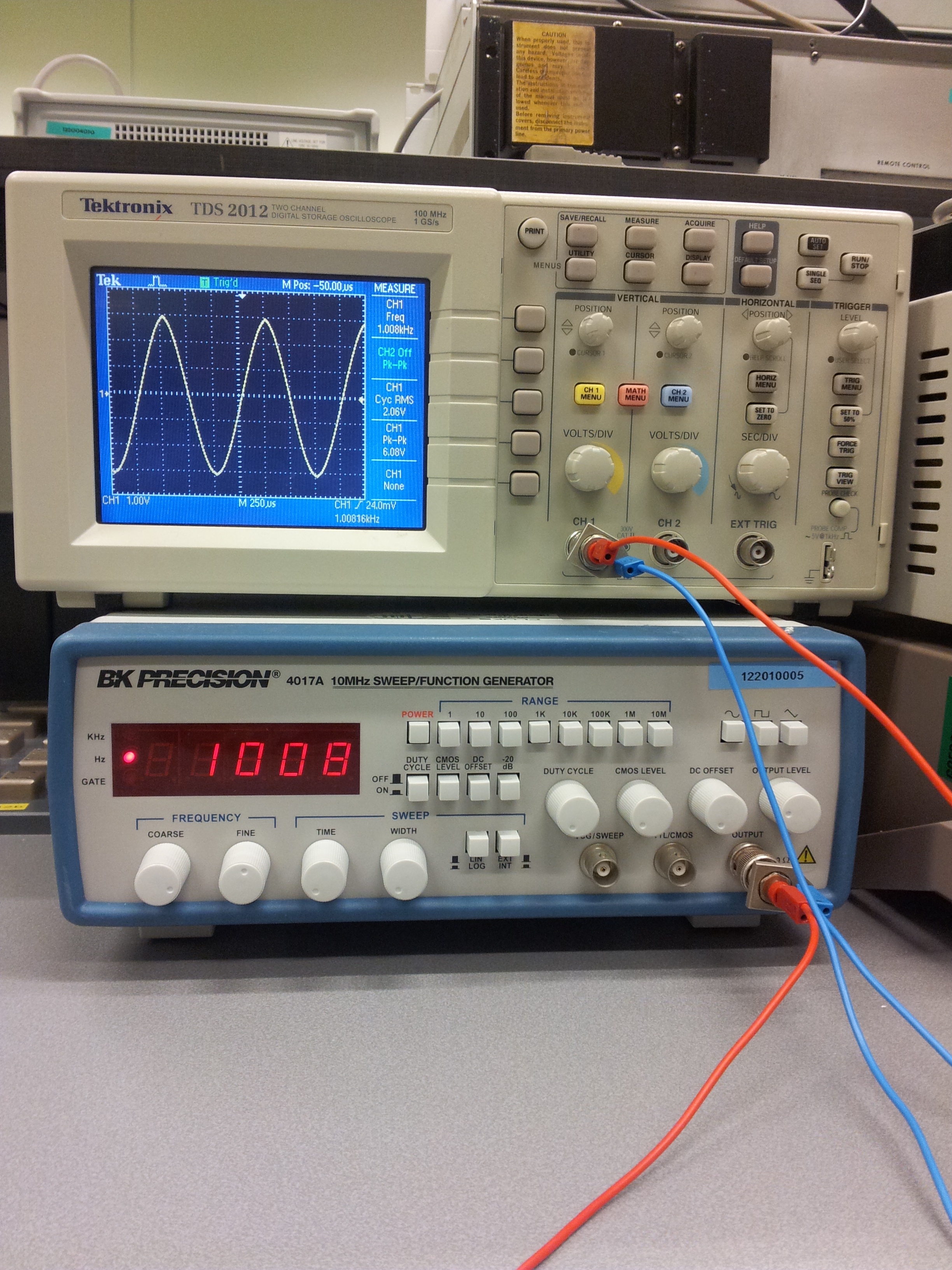
Investigate the use of the oscilloscope and triggering; Make a ‘frozen’ sine wave visible. Check the timebase of the oscilloscope and check if the frequency matches the frequency of the functiongenerator. Describe how you determined the frequency on the oscilloscope.

8.2.2.2. Assignment 2.

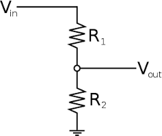
Use 2 resistors with values R1 = 10 k ohm and R2 = 100 k ohm. Connect the resistors as follows:

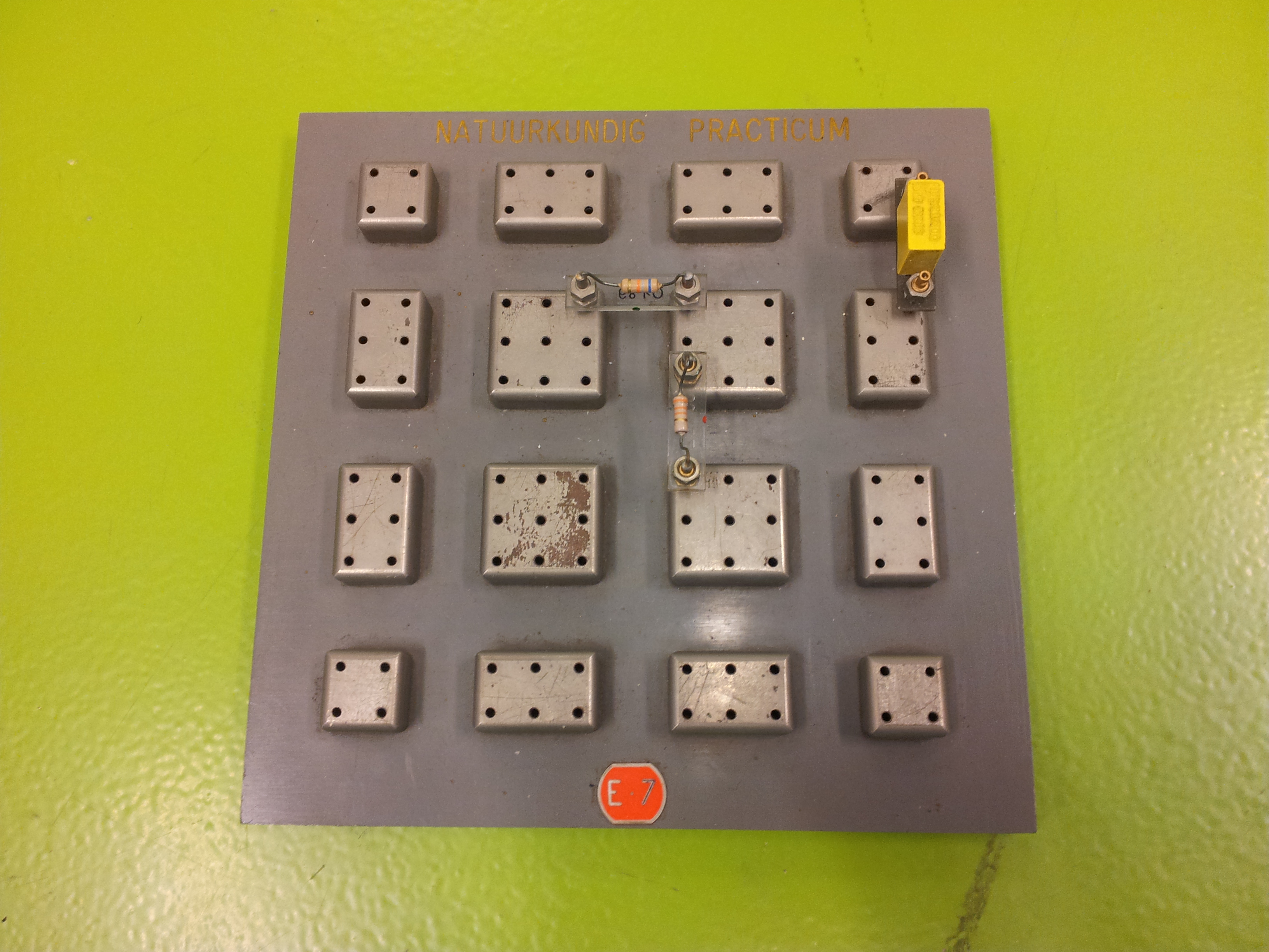
Use the metal connector board for the resistors:

Connect the sinewave signal from the functiongenerator to the input of our resistor network. Determine the \(\frac{U_{out}}{U_{in}}\) using Ohm’s law: U = I * R. Check if the factor is correct by using the oscilloscope (use two channels!)

8.2.2.3. Assignment 3

Connect a headphone parallel to R2. What do you see on the oscilloscope? Can you explain why the signal has become very small or disappeared?

Use an amplifier to amplify the signal. The amplifiers are in fact so-called differential amplifiers: Uout = A(Ain+ - Uin-), but by grounding one input you can use them to amplify one channel too. Check if it works by connecting the output to the oscilloscope. You will see a misformed signal. Can you explain this?

8.2.2.4. Assignment 4.

Replace in the network R1 by 100k and R2 by a capacitor of 1 nF.

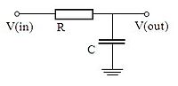
Read the description of the complex impedance in section 5.1.8 and 5.1.9 Analog Electronics. What can you say about the behaviour of this network?

Check the working by changing the frequency of the functiongenerator and listening through the headphone.

8.2.2.5. Assignment 5

Decibel (dB) is a logarithmic (!) unit to express the following:

\[H(dB) = 10 ^{10} log(|\frac{P_{out}}{P_{in}})|\]

with P the power of a signal. By using voltage we get:

\[A(dB) = 20 ^{10} log(|\frac{U_{out}}{U_{in}})|\]

Create a table of approximately 15-20 values for A(dB) using a frequencyband of 0-10 kHz and using the network above. Plot the amplitude on the vertical axis and frequency on the horizontal axis using matplotlib. Take care to use the correct representation... A typical characteristic of filters is the frequency where the proportion between output and input has decreased with a factor 2. Which frequency corresponds with this point. Check if this point is correct by calculating the timeconstant of the filter:

\[\omega = \frac{1}{RC}\]

8.2.2.6. Assignment 6

Perhaps you have already noticed that the input and output of the RC network has a phase difference. This phase difference can be measured using:

\[\phi = 2\pi \frac{\Delta t}{T} = 2\pi f \Delta t\]

By using the oscilloscope we can determine the phase difference. Create a table with phase difference in radians and plot the result in a second plot below you amplitude-frequency plot. The combination of both plots is called a “Bode diagram”.

8.2.2.7. Assignment 7

Before we dig into the world of digital filters it’s nice to see an analog filter which is still much used in many applications. It’s a so called Butterworth filter with a characteristic which we will also see in the digital variant. We will use an operational amplifier (“opamp”) and we have simple plugin modules with these small chips on a board where resistors and capacitors can be connected to the input and output of the amplifier. Please note: an opamp has a large gain of \(10^6\). The output is related to 2 inputs: \(U_o = A (U_i(+) - U_i (-))\): it amplifies the difference between 2 signals. Opamps are used always in a feedback circuit; we will see such systems later when we start with control theory. To understand the circuit it’s good to know that an ideal opamp has no current flowing into to amplifier (i.e. it has an infinite input impedance), only through the resistors and other components. When we connect to + input to ground we create a virtual ground point on the - input. (proof can be done by using Kirchhoff and Ohm’s laws). By using the feedback we get a system which is largely independent on impedances which are connected to output and input (within a certain range of course) and we can be represented by a simple algebraic equation.

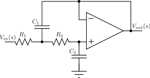
Use a resistor of 150k and capacitor of 1 nF and build this circuit. Scan with the oscilloscope through the frequencies. Check the circuit functionality.

8.2.2.8. Assignment 8

Add a second filter using opamps but with opposite behaviour in frequency. Try to math the cut-off frequency of the first circuit. What do you expect and do you see the behaviour?