8.2.3. Lab week 3: Fourier series, transformation and discrete signals
8.2.3.1. Assignment 1.
Sympy is a nice library for symbolmanipulation in Python and has some resemblance with Mathematica. Unfortunately it contains a few errors but the following assignment is possible.
from sympy.plotting import plot
from sympy import symbols

x = Symbols('x')
plot(x, x**2, x**3, (x, -5, 5))
from sympy import *
x = Symbol('x')
solve(x**2 - 3, x)
Please note that there is a difference between sympy.symbols and sympy.Symbol
Solve the following with sympy:
8.2.3.2. Assignment 2.
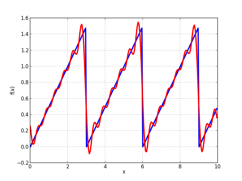
And now a bit more serious work with Fourier series. In controlsystems it’s interesting to see how a system behaves when we apply a certain input signal. Much used input signals are step (Heaviside), ramp (sawtooth) and pulse (dirac, this one can result in some problems with sympy by the way). Determine the Fourier response for those 3 signals using sympy and plot a few terms of the series for a short interval. Plot input AND output signal. The result should look like:
8.2.3.3. Assignment 3.
Write a Python function which creates a sine of 100 Hz and returns the samples with timing. Recreate the timedomain signal by using a Sinc and plot both functions. Experiment with different samplesarate above and below the Shannon frequency and show what happens.
8.2.3.4. Assigment 4.
Do the same for the following function:
Show what happens with different samplefrequencies.
8.2.3.5. Assignment 5.
The next file muziek_48kHz.wav contains a short piece of music in wav format. Using the ‘wave’ library of Python you can extract several interesting fields of this file:
wav_header_dtype = np.dtype([
 ("chunk_id", (str, 4)),
 ("chunk_size", "<u4"),
 ("format", "S4"),         # 4-byte string
 ("fmt_id", "S4"),
 ("fmt_size", "<u4"),
 ("audio_fmt", "<u2"),
 ("num_channels", "<u2"),
 ("sample_rate", "<u4"),
 ("byte_rate", "<u4"),
 ("block_align", "<u2"),
 ("bits_per_sample", "<u2"),
 ("data_id", ("S1", (2, 2))),
 ("data_size", "u4"),
 ])
Load the music using ‘readframes’ and perform a ‘downsampling’ by using only 1 sample of each 6 samples and create a new wav file. Play the wav file. Not very nice, as you will notice. What has happened? The correct way is using a resample function. On linux the easy route is using the program ‘sox’. Do a resampling to 8 kHz and compare the file with the original.
8.2.3.6. Assignment 6.
Download the following file containing EEG measurement data: :download: EEG data You will see that it is quite noisy. The file cotains samples of 16 samples and was sampled with 500 Hz. we are only interested in channel 1. Plot this channel and take care to have correct values on the axis. We can filter this signal using convolution from the numpy library using a window of ‘ones’:
window = np.ones(int(window_size))/float(window_size)
Plot the filtered signal with a different color and experiment with the window size. Start with 10 for instance.