1.2.3. Basic Signals
1.2.3.1. Constant Signal
That’s easy:
| CT | DT |
|---|---|
| \(x(t) = 1\) | \(x[n] = 1\) |
and of course we could use any constant instead of 1 (even complex valued constants).
1.2.3.2. Step Function
A step function is far more important and far more common then you might think. When you hit the light switch at time \(t=0\) and you think of the lamp as a system that is fed the electrical signal \(x(t)\) as input and outputs light (with measured intensity \(y(t)\)), this system is fed with a step function. For \(t<0\) there was no voltage difference at the lamp and then suddenly from time \(t=0\) and onwards the lamp is fed with a 230 V electrical signal.
What happens in the lamp system? When there is voltage applied to the lamp (we think of an old fashioned lamp) current starts to flow through the filament (a piece of wire) and the filament starts to heat up (filaments have the property to give a lot a light when heated). After a (short) while there is an equilibrium, the filament is at a constant temperature and thus the output \(y(t)\) is constant. But what happens between time \(t=0\) and the time the equilibrium settles in?
Yes the above explanation of a lamp turned on does fit into these lecture series. The transition the lamp makes from off to on is called the step response of the system. When we are looking at control theory at the end of these lectures series we will look into this at more detail.
| CT | DT |
|---|---|
| \(x(t) = \begin{cases} 0 &: t<0\\ 1 &: t\geq 0\end{cases}\) | \(x[n] = \begin{cases} 0 &: n<0\\ 1 &: n\geq 0\end{cases}\) |
1.2.3.3. Pulse Function
The pulse function, also called the impulse function, in DT is easy: everywhere zero except at \(n=0\) where the values is \(1\). The DT pulse is written as \(\delta[n]\).
In CT it is more difficult. The pulse in CT is written as \(\delta(t)\). It is mathematically defined with the sifting property:
Don’t worry in case you cannot make much sense out of this property. It is not even an (Stieltjes) integral that we are used to.
A usefull way to think about a pulse signal is to consider a signal in which you want to concentrate a finite amount of energy in a short a time interval as possible. Energy in a signal is measured by integrating a signal over a period of time.
Consider for instance the signal \(x_a(t)\) defined as:
The total energy in this signal is \(1\) (the integral of \(x(t)\) over the entire domain). This is true irrespective of the value of \(a\). In the limit when \(a\rightarrow0\) the value \(x_a(0)\rightarrow\infty\) but still the total area under the function remains 1. In a sloppy way we may define:
The strange thing thus is that the function value is infinite (well more accurate said it is not well defined) at \(t=0\) whereas the integral over the entire domain is finite and equal to 1.
We will see many uses of the pulse function. The translated CT pulse function \(3 \delta(t-2)\) is plotted as:
In [1]: n = np.arange(10);

In [2]: x = np.zeros_like(n);

In [3]: x[2]=3;

In [4]: plt.vlines(n,0,x,'b');

In [5]: plt.ylim(-1,4);

In [6]: plt.plot(n,0*n, 'b');

In [7]: plt.show();
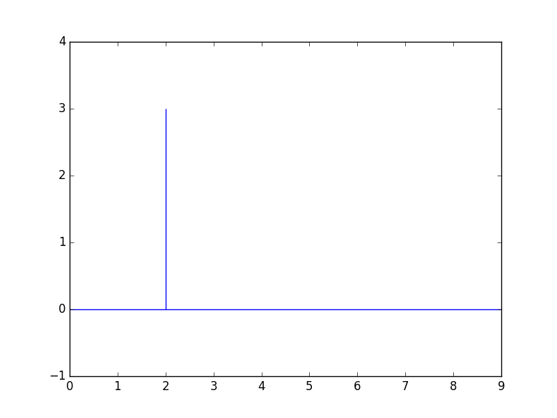
The straight line indicates it is a pulse and the length of the line indicates the total energy.
| CT | DT |
|---|---|
| \(x(t) = \delta(t) \equiv \lim_{a\rightarrow0} x_a(t)\) | \(x[n] = \delta[n] \equiv \begin{cases} 1 &: n=0\\ 0 &: \text{elsewhere} \end{cases}\) |