4. Overview of models and model equations

4.4 Quantum world

The pre-university physics (vwo) examination program contains the domain Quantum World.¹ This world is built on two fundamental models: the photon model of light and the quantum model of particles

1. Photon model of light
   An atom has a size of about 10^-1 nm. For wavelengths on this very small scale, electromagnetic radiation appears to behave in many respects as a collection of discrete particles. This was explained by Albert Einstein in 1905 by assuming that light consists of energy packages called 'photons', with energy proportional to the frequency \(f\) of light: $$E_{\rm f}=h\cdot f $$ The Planck constant \( h = 6{,}6 \cdot 10^{- 34} \rm{Js}\), named after the German physicist Max Planck, is the fundamental constant within the quantum world. In SI units the Planck constant has a very small value, but in the atomic world where all dimensions are very small, this constant dominates the physical phenomena.
2. Quantum model of particles
   Within an atom, the electrons are bound to the nucleus by electrical attraction. Virtually all observable properties of atoms and molecules can be explained from the assumption that electrons in this restricted space behave like standing waves. The fundamental relationship that links a wavelength to a particle property was given in 1924 by Louis de Broglie: $$\lambda_{\rm B} = \frac{h}{{m \cdot v}}$$ Mass and velocity are in the denominator of this formula for the particle in question. The wavelength so defined is called the 'de Broglie wavelength'.

These two models form the basis of quantum mechanics² as developed around 1925 by a number of physicists, in the first place by Werner Heisenberg, Erwin Schrödinger, and Max Born. Quantum mechanics appears to give very accurate results that math those found in numerous experiments and applications.

Working with quantum mechanical theory requires imagination and a lot of mathematical ingenuity. Nevertheless, the essence of the atomic structure can be clearly understood from simplified representations and models.^3,4 Below we give an overview of a number of models in the subdomain Quantum World in the physics syllabus on Quantum World and Relativity¹ with corresponding files for the Coach 7 modelling environment.⁵

Note

In the following computer models atomic dimensions and energies are scaled with respect to the characteristic length and energy scale of the problem. This simplifies the model equations and the numerical calculation because numerical values are then of order one. Moreover, it gives a better insight into the structure of the equations. Multiplication by the scale factors offers the opportunity to return to SI units or another unit system.
No strict scaling conditions are imposed on the wave functions calculated in the examples. In most cases, the amplitude is chosen with the pragmatic aim to make the essential characteristics of the wave function clearly visible in the graphs.

1. 1-D Schrödinger equation

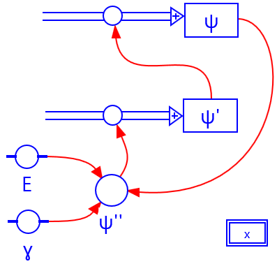
The wave that describes a quantum particle is called the 'wave function'. In the case of a quantum particle in a box, it is tacitly assumed that this wave function is given by a sine function \(\psi (x) = A \cdot \sin (k \cdot x)\) with amplitude \(A\) and wavenumber \(k=2\pi / \lambda\).
The calculation of the second derivative of this wave function gives the wave equation: \[\frac{{{d^2}\psi (x)}}{{d{x^2}}} = - {k^2} \cdot \psi (x)\] Substitution of the de Broglie relationship \(k= (2 \pi /h) m \cdot v \) leads to the Schrödinger equation (1-dimensional, stationary, i.e. time-independent) as presented on the right-hand side. Here, the total energy \(E\) is defined as the sum of the kinetic energy and potential energy \(V(x)\) of the quantum particle.
In the example below, a solution is calculated for a free quantum particle, i.e. \(V(x)=0\). There is a formal agreement with the model equations for the spring-mass model of harmonic motion 4.2.1 via the substitution \( u \to \psi\) and \(t \to x\text{.}\) The coordinate \(x\) normalised in the model equations via the de Broglie wavelength \(\lambda_{\rm B}\) and the energy is normalised with respect to the kinetic energy \(E_{\rm k}\) of the quantum particle.

Formulas in Binas:

$$\frac{{{d^2}\psi (x)}}{{d{x^2}}} + \frac{{8{\pi ^2} \cdot m}}{{{h^2}}}\left( {E - V(x)} \right) \cdot \psi (x)=0 $$ $$\begin{array}{l} E = \frac{1}{2} m \cdot {v^2} + V(x)\\ \lambda_{\rm B} = h / m \cdot v \end{array} $$

Difference equations:

$$\begin{array}{l} \psi '' = - \gamma \cdot \left( {E - V} \right) \cdot \psi \\ \Delta \psi ' = \psi '' \cdot \Delta x\\ \Delta \psi = \psi ' \cdot \Delta x \end{array}$$

Notation:

$$\begin{array}{l} \psi '': = d^2 \psi / dx^2 = d\psi '/dx\\ \psi ': = d\psi / dx\\ \gamma : = 2 m /\hbar^2 \\ \hbar : = h/ 2 \pi \end{array}$$

Dimensionless variables:

$$\begin{array}{l} x \to \lambda_{\rm B} \cdot x \quad \lambda_{\rm B}=\sqrt{2mE_k}/h \\ \psi'' \to \lambda_{\rm B}^{-2} \cdot \psi''\\ E \to E/E_{\rm k}\quad E_{\rm k}=(m\cdot v^2)/2\\ \gamma \to \lambda_{\rm B}^2 \cdot E_{\rm k}\cdot \gamma= (2\pi)^2 \end{array}$$

Text-based model

\(\begin{array}{l} \psi '' = - \gamma \cdot E \cdot \psi \\ \psi ' = \psi ' + \psi '' \cdot dx\\ \psi = \psi + \psi ' \cdot dx \\x=x+dx \end{array}\)

Graphical model



Coach 7

Coach 7

Example

Initial values

\(\begin{array}{l} \gamma = (2\pi)^2\\E=1\\ \psi'(0) =1\\\psi(0)=0\\x=0\\ dx=0{.}001 \end{array}\)


2. Quantum particle in a box

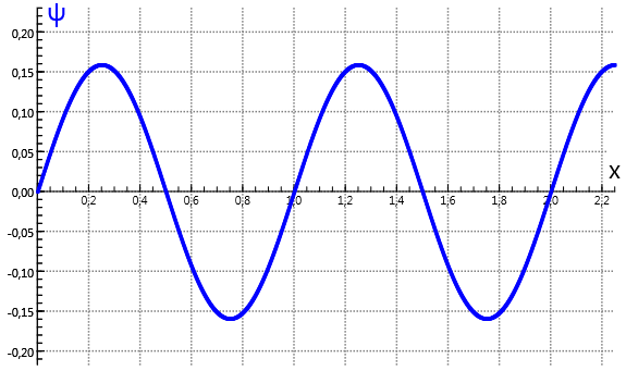
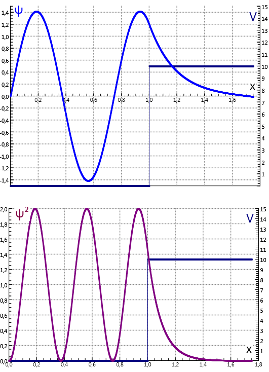
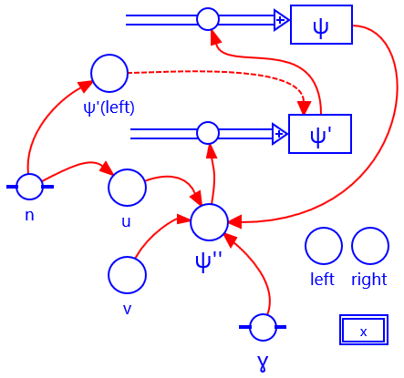
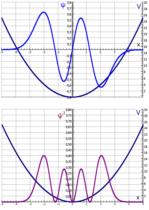
We consider a quantum particle captured in 1-dimensional infinitely deep well with potential \(V(x) = \infty \) if \( x < 0, x > L \). The potential energy is zero (\( V(x)=0\)) inside the well. The solution of the 1-dimensional Schrödinger equation is in that region a sine function.
This wave function \( \psi(x)\) must satisfy the boundary conditions \(\psi(0)=0,\psi(L)=0\), i.e. \( k \cdot L = \pi \cdot n, \, n = 1,2,3{,}...\). The admissible energy values follow from this as:⁶ $$ E_n = {E_1} \cdot {n^2}\quad {E_1} = \frac{{{\pi ^2}}}{{\gamma \cdot {L^2}}} = \frac{{{h^2}}}{{8m \cdot {L^2}}}$$ If the well has a dimension at nanoscale, for example \(L= 2 \rm{nm}\), a typical value for a quantum dot, and the mass is that of an electron, then the energy of the ground state is \({E_1} = 1{.}5 \cdot {10^{ - 20}}{\rm{J}}\). In SI units this is an inconveniently small number. That is why one commonly expresses the energy of atomic processes in electron volts: \({E_1} \approx 0{.}1\, {\rm{ eV}}\).
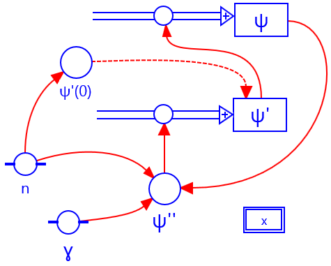
This model is computed below. The condition that the wave function must be zero at the boundaries is taken into account via the initial value of the energy. In the model equations the variables are dimensionless after scaling with the length \(L\) and the energy \(E_1\).

Formulas in Binas:

$$\frac{{{d^2}\psi (x)}}{{d{x^2}}} + \gamma \left( {E - V(x)} \right) \cdot \psi (x)=0 $$ $$\begin{array}{l} E = \frac{1}{2} m \cdot {v^2} + V(x)\\ \gamma = 8{\pi ^2} \cdot m / h^2 \end{array} $$

Difference equations:

$$\begin{array}{l} \psi '' = - \gamma \cdot \left( {E - V} \right) \cdot \psi \\ \Delta \psi ' = \psi '' \cdot \Delta x\\ \Delta \psi = \psi ' \cdot \Delta x \end{array}$$

Solution \(V=0\):

$$\psi(x) = A\sin(k \cdot x) \quad k = \sqrt {\gamma E}$$

Dimensionless variables:

$$\begin{array}{l} x \to L \cdot x \\ \psi'' \to L^{-2}\cdot \psi'' \\ n^2=E/E_1\\ \gamma \to L^2 \cdot E_1\cdot \gamma= \pi^2 \end{array}$$

Text-based model

\(\begin{array}{l} 0 \leq x \leq 1\\ \psi '' = - \gamma \cdot n^2 \cdot \psi \\ \psi ' = \psi ' + \psi '' \cdot dx\\ \psi = \psi + \psi ' \cdot dx \\x=x+dx \end{array}\)

Graphical model



Coach 7

Coach 7

Example

Initial values

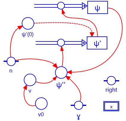
\(\begin{array}{l} n=3\\ \gamma=\pi^2\\\psi'(0) =\sqrt{2}\cdot n \cdot \pi\\\psi(0)=0\\x=0\\ dx=0{.}001 \end{array}\)


3. A box with one finite wall

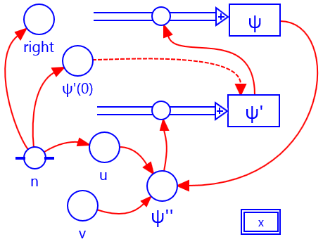
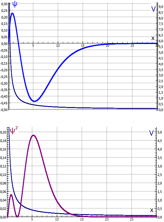
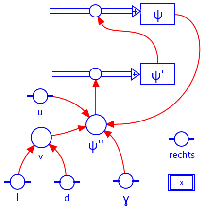
In this model, a quantum particle is located in a box with one finite wall. The potential is \(V(x) = \infty \) if \( x < 0 \) and \(V(x)=V_0\) if \(x > L \). The potential energy is zero \( (V(x)=0)\) inside the box. The solution of the 1-dimensional Schrödinger equation is in that region a sine function with wavenumber \(k = \sqrt {\gamma E}\). The solution of the Schrödinger equation outside the box, to the right, is an exponential function \({\psi _2}(x)\) with damping coefficient \(\kappa = \sqrt {\gamma ({V_0} - E)} \).
The admissible energy values can be computed numerically from the boundary conditions that the wave function and its derivative are continuous at the finite wall: \({\psi _1}(L) = {\psi _2}(L)\) and \( \psi{'_1}(L) = \psi{'_2}(L)\).⁷
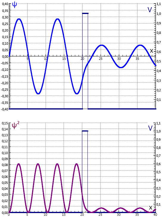
In the example below the eigenvalues are found by searching for wave functions that remain finite for certain values of \(E\). The parameters are the same as those in model 4.2.2 and we write for the energy \(E = {E_1} \cdot {n^2}\) where \(E_1\) is the energy of the ground state as found in 4.4.2; \(n\) is here a variable. By variation of the parameter value of \(n\) around 1 the ground state of a particle in a box with one finite wall can be found: \(n_1=0{.}90736\). In the same way we can compute excited states \(n_2, n_3\), as long as \( E-V_0 < 0\).
The model equations are simplified when one uses dimensionless variables. It turns out that the relative potential energy \(v_0\) is the determining parameter in this problem situation.

Formulas in Binas:

$$\frac{{{d^2}\psi (x)}}{{d{x^2}}} + \gamma \left( {E - V(x)} \right) \cdot \psi (x)=0 $$ $$\begin{array}{l} E = \frac{1}{2} m \cdot {v^2} + V(x)\\ \gamma = 8{\pi ^2} \cdot m / h^2 \end{array} $$

Difference equations:

$$\begin{array}{l} \psi '' = - \gamma \cdot \left( {E - V} \right) \cdot \psi \\ \Delta \psi ' = \psi '' \cdot \Delta x\\ \Delta \psi = \psi ' \cdot \Delta x \end{array}$$

Solution \(V=0\):

$$\begin{array}{l}\psi_1(x) = A\sin(k \cdot x) \\k = \sqrt {\gamma E} \end{array}$$

Solution \(V=V_0\):

$$\begin{array}{l}{\psi _2}(x) = F \exp(-\kappa \cdot x) \\ \kappa = \sqrt{\gamma ({V_0} - E)} \end{array}$$

Dimensionless variables:

$$\begin{array}{l} x \to L \cdot x \\ \psi'' \to L^{-2} \cdot \psi''\\ n^2=E/E_1\\ v_0=V_0/E_1\\ \gamma \to L^2 \cdot E_1\cdot \gamma= \pi^2 \end{array}$$

Text-based model

\(\begin{array}{l} 0 \leq x \leq {\rm right} \\ {\rm If} \; x > 1 \\ \quad {\rm Then} \; v=v_0 \\ \quad {\rm Else}\; v=0 \\ {\rm EndIf}\\ \psi'' = -\gamma\cdot (n^2 -v)\cdot\psi\\ \psi ' = \psi ' + \psi '' \cdot dx \\ \psi = \psi + \psi ' \cdot dx \\x=x+dx \end{array}\)

Graphical model



Coach 7

Coach 7

Example

Initial values

\(\begin{array}{l} n_1=0{.}90736\\ n_2=1{.}80646\\n_3=2{.}67850\\ n=n_3\\ \gamma=\pi^2\\v_0=10\\ \psi'(0)= \sqrt{2} \cdot n \cdot \pi\\ \psi(0) = 0\\x = 0\\ dx=0{.}001 \\ {\rm right} = 7/4 \end{array}\)


4. A finite symmetric well

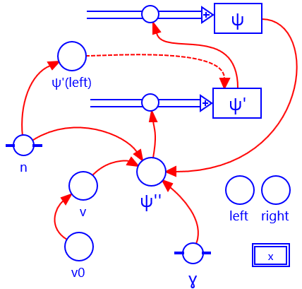
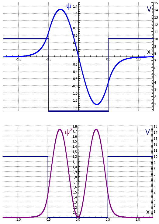
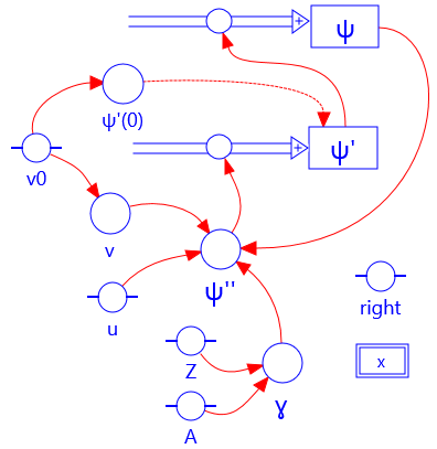
As a variant of model 4.4.3, a quantum particle is considered in a symmetrical 1-dimensional well with two finite walls. The potential is \(V(x)=V_0\) if \(|x| > L/2\text{.} \) The potential energy is zero (\( V(x)=0\)) inside the box \((|x| < L/2)\text{.}\) The wave function \(\psi_2(x)\) is in that region a linear combination of a sine and cosine function, with linear coefficients \(A\) and \(B\) that are determined from boundary conditions at the walls of the well and the normalisation. The solution of the Schrödinger equation outside the box is an exponential function \({\psi _{1,3}}(x)\) with parameters \(F\) and \(G\) that have to be determined yet.
The admissible energy values can be computed numerically from the boundary conditions that the wave function and its derivative are continuous at the finite walls: \({\psi _1}(-L/2) = {\psi _2}(-L/2)\), \( \psi{'_1}(-L/2) = \psi{'_2}(-L/2)\) and the same for \(\psi_{2,3}\) at \(L/2\).⁷
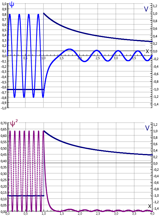
In the example below the numerical eigenvalues are found from the model equations. These rules can be simplified by switching to dimensionless variables, similarly as was done in model 4.4.3. \(E_1\) is the energy of the ground state of model 4.4.2, and the parameter values are the same as those in model 4.4.3.
The discrete eigenvalues can be determined by looking for solution that stay finite for particular values of \(n\). The ground state of a particle in a symmetric finite well can be found by variation of the parameter value of \(n\) around 1: \(n_1=0{.}83077\). In the same way we can compute excited state \(n_2, n_3\), as long as \( E-V_0 < 0\).

Formulas in Binas:

$$\frac{{{d^2}\psi (x)}}{{d{x^2}}} + \gamma \left( {E - V(x)} \right) \cdot \psi (x)=0 $$ $$\begin{array}{l} E = \frac{1}{2} m \cdot {v^2} + V(x)\\ \gamma = 8{\pi ^2} \cdot m / h^2 \end{array} $$

Difference equations:

$$\begin{array}{l} \psi '' = - \gamma \cdot \left( {E - V} \right) \cdot \psi \\ \Delta \psi ' = \psi '' \cdot \Delta x\\ \Delta \psi = \psi ' \cdot \Delta x \end{array}$$

Solution \( x < -L/2\):

$$\begin{array}{l}{\psi _1}(x) = G\exp(\kappa \cdot x) \\ \kappa = \sqrt {\gamma ({V_0} - E)} \end{array}$$

Solution \( |x| < L/2\):

$$\begin{array}{l}\psi_2(x) = A\sin(k \cdot x) + B\cos(k\cdot x)\\k = \sqrt {\gamma E} \end{array}$$

Solution \(x > L/2 \):

$$\begin{array}{l}{\psi _3}(x) = F\exp(- \kappa \cdot x) \\ \kappa = \sqrt {\gamma ({V_0} - E)} \end{array}$$

Dimensionless variables:

$$\begin{array}{l} x \to L \cdot x \\ \psi''\to L^{-2} \cdot \psi''\\ n^2=E/E_1\\ v_0=V_0/E_1\\ \gamma \to L^2 \cdot E_1\cdot \gamma= \pi^2 \end{array}$$

Text-based model

\(\begin{array}{l} {\rm If} \; x < -0{.}5\; \rm{or} \; x > 0{.}5\\ \quad {\rm Then} \; v=v_0\\ \quad {\rm Else}\; v=0\\ {\rm EndIf}\\ {\rm If}\, (\rm{left} < x) \, \rm{and}\, (x < \rm{right})\\ \quad {\rm Then}\\ \psi '' = - \gamma \cdot (n^2-v) \cdot \psi \\ d\psi ' = \psi '' \cdot dx\\ d\psi = \psi ' \cdot dx\\ \quad {\rm Else}\\ d\psi '=0\\ d\psi=0\\ {\rm EndIf}\\ \psi' = \psi' + d\psi'\\ \psi = \psi + d\psi \\x=x+dx \end{array}\)

Graphical model



Coach 7

Coach 7

Example

Initial values

\(\begin{array}{l} {\rm left}=-5/4 \\{\rm right}=5/4 \\n_1=0{.}83077\\ n_2=1{.}65044\\n_3=2{.}43928\\n=n_2\\ \gamma=\pi^2\\v_0=10\\ \psi'(\rm left) = 1/(-1000+2500 \cdot n - 750\cdot n^2)\\ \cdot 1{.}1\cdot n^2 \cdot \sqrt{2\cdot n \cdot \pi} \\ \psi' =\psi'(\rm left)\\\psi=0\\x={\rm left}\\ dx=0{.}001 \end{array}\) \(\begin{array}{l} \end{array}\)


5. Harmonic oscillator

The potential energy is in model 4.4.4 a straight well. In many situations it is more realistic to assume that surrounding atoms bind a quantum particle in a harmonic potential well as if the particle is a mass on a spring; see model 4.2.1. In this case the 1-dimensional Schrödinger equation can be solved analytically.⁸ The discrete energy values are found as $$\begin{array}{l} E_n =E_0\cdot(2n + 1)\quad E_0=\frac{1}{2} h\cdot f_{\rm v} \\ n=0{,}1{,}2{,}\ldots\end{array}$$ where \(f_{\rm v}=\sqrt{(C/m)}/2\pi\) is the frequency of the oscillatory motion of the spring-mass system. From the analytical solution it also follows that the system has a characteristic de Broglie wavelength \(\lambda_0=\sqrt{h/(m \cdot f_{\rm v})}/2\pi\).
The model equations⁶ are simplified by scaling length and energy with \(\lambda_0\) and \( E_0\). The discrete energy values can be determined numerically by variation of the variable \(u\). The condition is that the wave functions remain finite for these values and go to zero far from the origin. The initial value in the example below corresponds with the state \(n=3\).

Formulas in Binas:

$$\frac{{{d^2}\psi (x)}}{{d{x^2}}} + \frac{{8{\pi ^2} \cdot m}}{{{h^2}}}\left( {E - V(x)} \right) \cdot \psi (x)=0 $$ $$V(x)= \frac{1}{2}C \cdot x^2 $$

Difference equations:

$$\begin{array}{l} \psi '' = - \gamma \cdot \left( {E - V} \right) \cdot \psi \\ \Delta \psi ' = \psi '' \cdot \Delta x\\ \Delta \psi = \psi ' \cdot \Delta x \end{array}$$

Dimensionless variables:

$$\begin{array}{l} x \to \lambda_0 \cdot x \\ \psi'' \to \lambda_0^{-2}\cdot \psi''\\ u=E/E_0\\ \gamma \to \lambda_0^2 \cdot E_0\cdot \gamma= 1 \\V \to (C\cdot \lambda_0^2/2E_0)\cdot x^2=x^2\end{array}$$

Text-based model

\(\begin{array}{l} V=x^2\\ {\rm If}\, (\rm{left} < x) \, \rm{and}\, (x < \rm{right})\\ \quad {\rm Then}\\ \psi '' = - \gamma \cdot (u-V) \cdot \psi \\ d\psi ' = \psi '' \cdot dx\\ d\psi = \psi ' \cdot dx\\ \quad {\rm Else}\\ d\psi '=0\\ d\psi=0\\ {\rm EndIf}\\ \psi' = \psi' + d\psi'\\ \psi = \psi + d\psi \\x=x+dx \end{array}\)

Graphical model



Coach 7

Coach 7

Example

Initial values

\(\begin{array}{l} {\rm left}=-5 \\{\rm right}=5 \\n=3\\ \gamma=1\\u=2n+1\\ \psi'(\rm left) = 0{.}000035\cdot {7^n}/\sqrt{2n!}\\ \psi' =\psi'(\rm left)\\\psi=0\\x={\rm left}\\ dx=0{.}001 \end{array}\) \(\begin{array}{l} \end{array}\)


6. Hydrogen atom

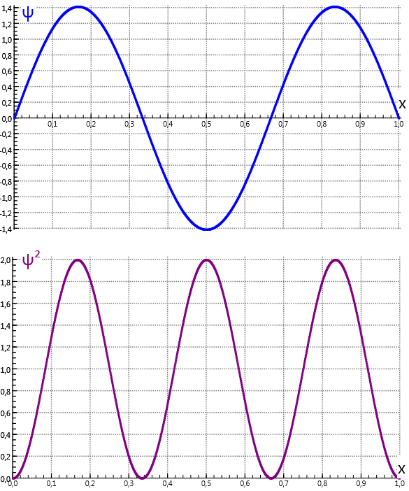
The electron and the proton in a hydrogen atom experience the attraction of the Coulomb force. As with a quantum particle in a well, the energy states of the hydrogen electron are quantized:⁶ $${E_n} = - \frac{R_{\rm y}}{n^2}\quad n=1{,}2{,}3...$$ where \( R_{\rm y}=13{.}61\,{\rm{eV}}\) is the Rydberg energy. The larger \(n\), the closer the energy levels are together. In quantum mechanics, the hydrogen electron is described with a wave function \(\psi\). The probability to find the electron at a distance \(r\) from the nucleus is given by the square of the wave function \(\left| \psi (r) \right|^2\). In the ground state, the maximum distance is the 'Bohr radius' \( a_0 \simeq 5{.}29 \cdot 10^{- 2}\rm{nm}\), as is computed in the example.⁹ The model equations are simplified when one uses dimensionless variables.

Formulas in Binas:

$$\frac{{{d^2}\psi (r)}}{{d{r^2}}} + \gamma \left( {E + f \frac{{{e^2}}}{r}} \right) \cdot \psi (r)=0 $$ $$\begin{array}{l} f= 1/4\pi \varepsilon_0\\ \gamma = 8{\pi^2} \cdot m / h^2\\ \end{array} $$

Difference equations:

$$\begin{array}{l} \psi '' = - \gamma \cdot \left( {E + f\cdot e^2/r } \right) \cdot \psi \\ \Delta \psi ' = \psi '' \cdot \Delta r\\ \Delta \psi = \psi ' \cdot \Delta r \end{array}$$

Hydrogen atom:

$$\begin{array}{l}a_0= h^2/(4\pi^2f \cdot {e^2}\cdot {m_e}) \\ E_1 = - f \cdot e^2 / 2 a_0=-R_{\rm y}\\ {a_0}^2\cdot R_{\rm y}\cdot \gamma=1 \end{array}$$

Dimensionless variables:

$$\begin{array}{l}x= r /a_0 \\ u^2= -E/R_{\rm y} \end{array}$$

Text-based model

\(\begin{array}{l} 0 < x \leq {\rm right} \\ v=2/x \\ \psi '' = (u^2 - v) \cdot \psi \\ \psi ' = \psi ' + \psi '' \cdot dx\\ \psi = \psi + \psi ' \cdot dx\\x=x+dx \end{array}\)

Graphical model



Coach 7

Coach 7

Example

Initial values

\(\begin{array}{l} n=2\\{\rm right}=15n\\ u=1/n \\ \psi'(0) = 2/\sqrt{n^3}\\ \psi(0)=0\\x=0{.}0000000001\\ d=0{.}001 \end{array}\)


7. Quantum tunneling

Quantum particles can pass potential barriers that cannot be penetrated according to classical mechanics. The explanation for this effect of ‘tunneling’ is the fact that the wave function is not zero but decreases exponentially in case of a finite energy barrier; see models 4.4.3-4.4.6.
As a simple model, for example for a scanning tunneling microscope (STM) ^6,10, we consider an energy barrier of height \(V=V_0\) and width \(D\). A quantum particle can move freely with energy \(E > 0\) in the area \(x < L \) left of the barrier and the area \( L+D < x \) right of the barrier. The wave functions \(\psi_{1,3}\) are in these areas linear combinations of sine and cosine functions. Inside the barrier holds \(E < V_0\) and the solution is there an exponential function \( \psi _{2}\). The normalisation constants are determined by the conditions that the wave function and its derivative are continuous at the walls of the barrier.¹¹
The conclusion is that the probability \(|\psi_3|^2 \) of finding the particle to the right of the potential barrier has a finite value. The transmission coefficient which gives the probability that a particle tunnels to the outside is in case \(\kappa \cdot D \gg 1\) approximated¹² by $$ T \simeq \frac{{|{\psi _2}(L+D)|{}^2}}{{|{\psi _2}(L){|^2}}} = \exp - 2\kappa \cdot D $$ A higher and wider barrier implies a (much) smaller probability.
This simple model is computed in the example below. Left and right of the barrier, the quantum particle is considered free \(E > 0\), but inside the barrier holds \(E < V_0\). In the model equations we scale the horizontal coordinate by the length \( {x_0} = \sqrt {1/\gamma \cdot {V_0}} \), which is a measure of the distance over which the wave function decays in the barrier; the relevant energies are scaled by the height of the barrier \({V_0}\).

Formulas in Binas:

$$\frac{{{d^2}\psi (x)}}{{d{x^2}}} + \gamma \left( {E - V(x)} \right) \cdot \psi (x)=0 $$ $$\begin{array}{l} E = \frac{1}{2} m \cdot {v^2} + V(x)\\ \gamma = 8{\pi ^2} \cdot m / h^2 \end{array} $$

Difference equations:

$$\begin{array}{l} \psi '' = - \gamma \cdot \left( {E - V} \right) \cdot \psi \\ \Delta \psi ' = \psi '' \cdot \Delta x\\ \Delta \psi = \psi ' \cdot \Delta x \end{array}$$

Solution \( x < L\):

$$\begin{array}{l}\psi_1(x) = A\sin( k \cdot x) + B\cos(k\cdot x)\\k = \sqrt {\gamma E} \end{array}$$

Solution \( L < x < L+D\):

$$\begin{array}{l}{\psi _2}(x) = F\exp(- \kappa \cdot x) \\ \kappa = \sqrt {\gamma ({V_0} - E)} \end{array}$$

Solution \(x > L+d \):

$$\begin{array}{l}\psi_3(x) = G\sin(k\cdot x) + H\cos(k\cdot x)\\k = \sqrt {\gamma E} \end{array}$$

Dimensionless variables:

$$\begin{array}{l} x \to x_0 \cdot x \quad x_0=1/\sqrt{\gamma V_0}\\ \psi'' \to x_0^{-2}\cdot \psi'' \\ l= L/x_0 \\d=D/x_0\\ u=E/V_0\\ v=V/V_0\\ \gamma \to x_0^2 \cdot V_0 \cdot \gamma = 1 \end{array}$$

Text-based model

\(\begin{array}{l} 0 \leq x \leq \rm{right} \\ {\rm If}\: (x > l)\, {\rm and}\, (x < l+d)\\ \quad {\rm Then} \quad v=1\\ \quad {\rm Else} \quad v=0\\ {\rm EndIf}\\ \psi''= - \gamma\cdot (u-v) \cdot \psi \\ \psi ' = \psi ' + \psi '' \cdot dx\\ \psi = \psi + \psi ' \cdot dx \\ x=x+dx \end{array}\)

Graphical model



Coach 7

Coach 7

Example

Initial values

\(\begin{array}{l} {\rm right}=40\\\gamma=1\\ l=20\\d=1{.}5\\u= 0{.}355658\\ \psi'(0) = 0{.}17\\\psi(0)=0\\x=0\\ dx=0{.}001 \end{array}\)


8. Alpha decay

Quantum tunneling is the basis for the statement by George Gamow in 1928 about the phenomenon that heavy nuclei show alpha decay:^13,14 $${}^A {\rm{X}}_Z \to {}^{A - 4}{\rm{Y}}_{Z - 2} + {}^4{\alpha}_2$$ By tunneling, an alpha particle (two neutrons and two protons) can escape the strong force within the atomic nucleus. The assumption is that in the nucleus of a radioactive isotope, an alpha particle can move more or less freely with the same energy as that of the alpha particle emitted, namely \({E_\alpha } \sim 4 - 9{\rm{MeV}}\). The combination of nuclear force and the repulsive Coulomb force creates a potential barrier. The higher the atomic number \(Z\) of the nucleus, the higher the Coulomb barrier. In the example, the nucleus is represented as a rectangular energy well \(V(r)=-V_{0},\; r < R_0\).^11,13 The radius of the nucleus is after decay equal to \({R_0} = 1{.}25{(A-4)^{1/3}} \cdot {10^{ - 15}}{\rm{ m}}\) with mass number \(A\). Outside the nucleus \(r \geq {R_0}\) the alpha particle is subject to the Coulomb repulsion $$V_{\rm c}(r) = \frac{1}{4\pi \varepsilon_0} \frac{2{e^2}(Z-2)}{r}$$ For distances greater than \(R_1\) determined by the equation \({V_{\rm c}}(R_1) = E_\alpha\), the kinetic energy is greater than the potential energy and the particle has escaped the nucleus.

Formulas in Binas:

$$\frac{{{d^2}\psi (r)}}{{d{r^2}}} + \gamma \left( {E - V(r)} \right) \cdot \psi (r)=0 $$ $$\begin{array}{l} E = \frac{1}{2} m \cdot {v^2} + V(r)\\ \gamma = 8{\pi ^2} \cdot m / h^2 \end{array} $$

Difference equations:

$$\begin{array}{l} \psi '' = - \gamma \cdot \left( {E - V} \right) \cdot \psi \\ \Delta \psi ' = \psi '' \cdot \Delta r\\ \Delta \psi = \psi ' \cdot \Delta r \end{array}$$

Solution \( r < R_0\):

$$\begin{array}{l}\psi_1(r) = A\sin(k \cdot r) + B\cos(k\cdot r)\\k = \sqrt {\gamma (E+V_{0})} \end{array}$$

Approximate solution \( R_0 < r < R_1 \):¹⁰

$$\begin{array}{l}{\psi _2}(r) \sim \exp(- \int_{{R_0}}^{{r}} {\kappa (\tilde{r})d\tilde{r}}) \\ \kappa (r) =\sqrt {\gamma (V_{\rm c}(r)-E)} \end{array}$$

Dimensionless variables:

$$\begin{array}{l} x = r/R_0\\ \psi'' \to R_0^{-2}\cdot \psi'' \\ u=E_{\alpha}/V_{\rm c}(R_0) = R_0/R_1 \\v=V/V_{\rm c}(R_0)\\ \gamma \to R_0^2 \cdot V_{\rm c}(R_0) \cdot \gamma = 0{.}69 (A-4)^{1/3}\cdot (Z-2) \end{array}$$

Text-based model

\(\begin{array}{l} 0 \leq x \\ {\rm If}\: x < 1\\ \quad {\rm Then} \quad v=- v_{0}\\ \quad {\rm Else} \quad v=1/x\\ {\rm EndIf} \\ \psi''= - \gamma \cdot (u-v) \cdot \psi \\ \psi ' = \psi ' + \psi '' \cdot dx\\ \psi = \psi + \psi ' \cdot dx \\ P=\psi^2\\x=x+dx \end{array}\)

Graphical model



Coach 7

Coach 7

Voorbeeld

Initial values

\(\begin{array}{l} \rm{right}=4\\A=210\\Z= 84\\\gamma = 0{.}69\cdot (A-4)^{1/3}\cdot (Z-2)\\ v_{0}=1{.}01297 \\u= 0{.}7\\ \psi'(0) = 10 + 9\sqrt{v_0}\\\psi(0)=0\\ dx=0{.}001 \end{array}\)