1.5. Image Representation
1.5.1. Coordinates and Indices
Accustomed to the choice of coordinate axes in mathematics you might think that the axes for an image \(f(x,y)\) are the same: the x-axis running from left to right, the y-axis from bottom to top with the origin in the lower left corner. This is not true for digital images in general (the one exception i know of is Microsofts Device Independent Bitmap).
In order to get an understanding of the many different formats for digital images we have to distinguish:
- the axes with the coordinates along those axes, and
- the indices into the array representing all samples.
We will use numpy and matplotlib throughout to set our definition for these lecture notes.
We will use this image as leading example:
In numpy this is easy to generate and plot with matplotlib:
In [1]: f = np.arange(12).reshape(3,4)

In [2]: plt.imshow(f, cmap='gray', interpolation='nearest');

In [3]: plt.show()
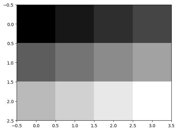
The sample points are in the middle of the squares (NOT pixels) and we see that the origin with coordinates is chosen to be at the top left. The x-coordinate axis runs from left to right and the y-coordinate axis runs from top to bottom.
In this coordinate axes system we can draw a line from \((0,2)\) to \((3,0)\)
In [4]: f = np.arange(12).reshape(3,4)

In [5]: plt.imshow(f, cmap='gray', interpolation='nearest');

In [6]: plt.plot([0,3], [2,0], lw=3);

In [7]: plt.show()
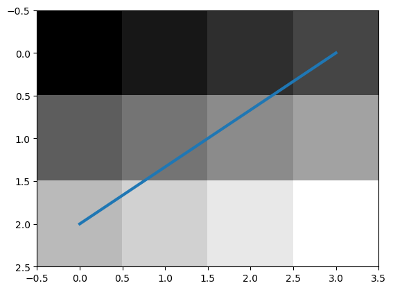
Carefully note that the coordinate system is a left-handed one. You have to turn the x-axis clockwise to the y-axis. The classical choice with x axis from left to right and y-axis from bottom to top results in a right-handed coordinate system. Be aware that in a left handed system things are a bit different then you might expect. A rotation over a positive angle \(\phi\) characterized with rotation matrix:
is turning a vector counter clockwise in a right handed coordinate system, but clockwise in a left handed system.
Being familiar with numpy arrays you have probably understood that in
case we want to index the array with the coordinates \((x,y)\) (with \(x\)
and \(y\) integer valued of course) that we need to write f[y,x].
So, the first index in the image array is the y-coordinate, and the second index is the x-coordinate.
1.5.2. Color Images
Let’s read a color image from disk and display it:
In [8]: f = plt.imread('python/data/images/peppers.png')

In [9]: plt.imshow(f);

In [10]: plt.show();

In [11]: print(f.shape)
(256, 256, 3)
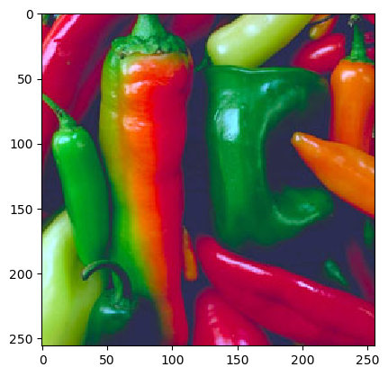
The shape of a color image array thus is \(M\times N \times 3\). It is also possible that a 4-th channel is used that encodes the transparency mask when displaying an image. Be sure to check and not assume things that are not nescessarily true.
Each of the planes f[:,:,c] with c equal to 0, 1 or 2
gives one of the color planes. Each color plane is a scalar image and
can be displayed as such:
In [12]: plt.imshow(f[:,:,1], cmap='gray'); # the green channel is a good approximation of the luminance

In [13]: plt.show()
