Chapter 2 Saddle-node bifurcation in a two-sexes population growth model
Here I formulate a model for a population that reproduces by means of sexual reproduction. Unlike the exponential and logistic growth model, this one is not an established population dynamic model that has been widely used in the population biological literature. Rather, it is introduced here mainly to illustrate some techniques for model analysis. The assumptions on which this model is based and its mathematical form are also much more debatable than those of the logistic growth model.
To model a population with sexual reproduction it is necessary to derive a mathematical representation for the process of two individuals encountering each other, mating and producing one or more offspring. Especially how to describe the rate at which encounters between sexual partners take place is not an easy or straightforward task. I follow an approach that has a long history in the modeling of chemical reactions: when two compounds \(A\) and \(B\) in a dilute gas or a solution react to yield a product \(C\), the rate at which this chemical reaction takes place is assumed to be proportional to the densities of both reactants \(A\) and \(B\). Hence, for the chemical reaction \[ A\;+\;B\quad\longrightarrow\quad C \] the rate with which the product \(C\) is produced is proportional to \[ [A]\cdot[B] \] where \([\,]\) refers to the concentration of a substance in the medium. The assumption that the rate of product formation is proportional to the product of the reactant concentrations has become known as the law of mass action or mass action law. Two requirements for it to hold is that the reactants move about randomly and are uniformly distributed through space.
Analogously to this approach from chemical reaction kinetics, I assume that the rate at which sexual partners encounter each other is proportional to the product of their abundance. If I furthermore assume that the sex ratio in the population is constant, the rate of encounter is proportional to the squared abundance \(N^2\). On encounter I assume that the partners produce offspring at a rate that decreases linearly with the population abundance \(N\). Hence, population reproduction can be described by a term \[ \beta\,N^2\,\left(1\,-\,\dfrac{N}{\Gamma}\right) \] in which the term \(N/\Gamma\) is the density dependent reduction in offspring production and \((1-N/\Gamma)\) hence is the realized fraction of the maximum offspring production (\(\beta\,N^2\)). To describe the death of individuals I simply assume that the rate of mortality equals \(\delta\). The rate at which individuals disappear from the population through death hence equals \(\delta N\). Putting these model pieces together, the dynamics of a population reproducing by means of sexual reproduction could therefore be described by the following ODE: \[\begin{equation} \dfrac{d\,N}{d\,t} = \beta\,N^2\,\left(1\,-\,\dfrac{N}{\Gamma}\right)\;-\;\delta\,N \tag{2.1} \end{equation}\]
The right-hand side of this equation can be represented with a function \(g(N)\) of the population density \(N\) with \(g(N)\) defined as: \[\begin{equation} g(N) = \beta\,N^2\,\left(1\,-\,\dfrac{N}{\Gamma}\right)\;-\;\delta\,N \tag{2.2} \end{equation}\] such that the model can be written as \[\begin{equation} \dfrac{dN}{dt} = g(N) \end{equation}\] where \(g(N)\) represents the population growth rate.
2.1 Equilibrium analysis
First we try to sketch a graph of the function \(g(N)\) (see (2.2)) as a function of its argument \(N\). This will allow us to assess for which values of \(N\) the population growth rate \(g(N)\) is positive (negative) and hence lead to an increase (decrease) in the population density \(N\). How to do this is the subject of basic function analysis and will not be discussed here in detail. The points to note about the function \(g(N)\) are:
the growth rate \(g(N)\) equals 0 for \(N=0\) (as should be the case for any dynamic model of a closed population),
for non-zero, but very small, positive values of \(N\) \(g(N)\) decreases to negative values,
for very large values of \(N\) the value of \(g(N)\) becomes very large, but negative, and
as long as
\[ \beta\,\Gamma\;>\;4\,\delta \] the function \(g(N)\) has two additional roots for which \(g(N)=0\). These roots will be indicated with the symbols \(\tilde{N}^{-}\) and \(\tilde{N}^{+}\), respectively.
Altogether, this leads to the following qualitative graph of \(g(N)\) as a function of \(N\), as shown in figure 2.1.
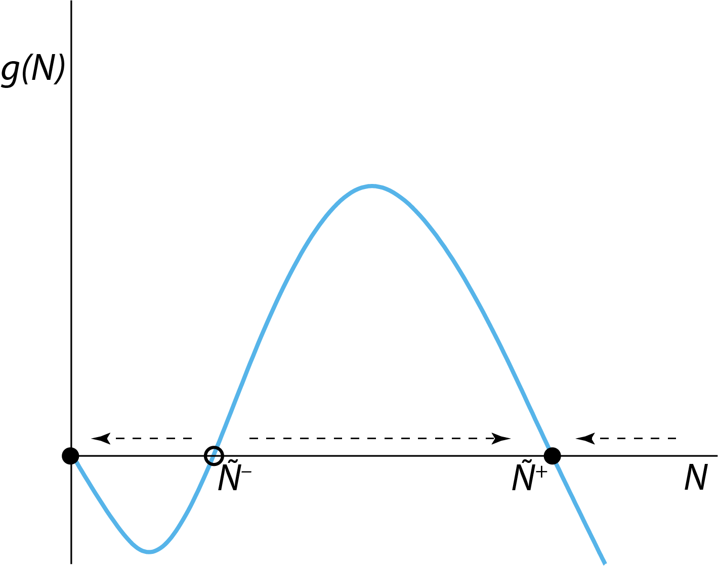
Figure 2.1: The right-hand side \(g(N)\) of the ODE describing the dynamics of the two-sexes population growth model. The horizontal arrows indicate for which values of \(N\) the population growth rate is negative (left-pointing arrows) and positive (right-pointing arrows) and the population abundance \(N\) will therefore decrease or increase over time. The open circle indicates the unstable steady state \(N=\tilde{N}^{-}\), closed circles indicate the stable steady states \(N=0\) and \(N=\tilde{N}^{+}\).
From this graph we can infer that the two-sexes population model has 3 steady states, where \(g(N)=0\). These steady states will be referred to as \(N=0\), \(N=\tilde{N}^{-}\) and \(N=\tilde{N}^{+}\), respectively. Note that a steady state of any dynamical system is characterized by the fact that the state of the system (in this population growth model the variable \(N\) representing the population abundance) will not change if the system starts out exactly in this steady state. That the system state will not change means that derivatives are 0, which in this population growth model implies that \(dN/dt=g(N)\) equals 0. Therefore, if the population would initially have an abundance equal to any one of the three values \(N=0\), \(N=\tilde{N}^{-}\) or \(N=\tilde{N}^{+}\), it would keep the particular abundance for all times. However, figure 2.1 also shows that not all of these 3 steady states are stable. For example, if the population abundance is perturbed away from \(N=0\) to a small positive abundance, its growth rate \(dN/dt=g(N)\) will be negative. Hence, it will decrease and approach \(N=0\) again. The steady state \(N=0\) is therefore stable. Similarly, if the population abundance is perturbed away from \(N=\tilde{N}^{+}\) to a slightly larger value, it will also have a negative growth rate, hence decrease and approach \(N=\tilde{N}^{+}\) anew. If perturbed away from \(N=\tilde{N}^{+}\) to a slightly smaller value, the population growth rate will be positive and \(N=\tilde{N}^{+}\) is approached as well. The steady state \(N=\tilde{N}^{+}\) is therefore also stable.
The steady state \(N=\tilde{N}^{-}\) is an entirely different matter: if perturbed away from this abundance to a slightly smaller value of \(N\), the population growth rate will be negative and the abundance will decrease and eventually approach the steady state \(N=0\). On the other hand, if perturbed away from this abundance to a slightly larger value, the population growth rate will be positive and the abundance will increase to eventually approach the steady state \(N=\tilde{N}^{+}\). The steady state \(N=\tilde{N}^{-}\) hence is an unstable steady state, because whenever the population abundance is perturbed away from this steady state, it will only move farther and farther away. In addition, it has the character of a breakpoint: it separates values of \(N\) that would eventually lead to approaching the stable steady state \(N=0\) from those values of \(N\) that would eventually lead to approaching the stable steady state \(N=\tilde{N}^{+}\). An unstable steady state like the one \(N=\tilde{N}^{-}\) encountered here is called a saddle point.
The horizontal arrows in figure 2.1 are drawn to indicate for which values of \(N\) the population growth rate \(g(N)\) is negative (left-pointing arrows) and positive (right-pointing arrows) and the population abundance \(N\) will therefore decrease or increase over time.
From figure 2.1 we can also deduce that at stable steady states the curve of \(g(N)\) as a function of \(N\) has a negative slope, while at unstable steady states (i.e. saddle points) the slope of \(g(N)\) is positive (Note, however, that this only holds as long as we are analyzing a model in terms of a single ordinary differential equation (ODE)).
Two more points can be deduced from the graphs presented here:
Every stable steady state has a basin of attraction.
Basin of attraction is the technical term for those initial states of a population dynamic model that would eventually lead to the particular steady state considered. Hence, the basin of attraction of the stable steady state \(N=0\) are all those population abundances for which \[ 0 < N < \tilde{N}^{-} \] while the basin of attraction of the stable steady state \(N=\tilde{N}^{+}\) are all those population abundances for which \[ N > \tilde{N}^{-} \] The boundary between the basins of attraction of two different, stable steady states is referred to as a separatrix. When, as in the cases considered here, the model is only one-dimensional (meaning it consists of only a single ODE) a separatrix is only a single point, which in the two-sexes population model considered here, corresponds to the saddle point \(N=\tilde{N}^{-}\). If the model is, however, of higher dimensions (i.e. described by more ODEs) separatrices can be lines, (curved) planes or even more complicated geometrical objects.The stability of a stable steady state may only be a relative concept
If the population abundance would initially be in the stable steady state \(N=\tilde{N}^{+}\), but would be drastically perturbed to a value below \(N=\tilde{N}^{-}\), the population abundance would approach the other stable steady state \(N=0\). Hence, that a steady state is stable against perturbations only holds for small perturbations that do not bring the abundance outside the basin of attraction of the steady state. Mathematically, we therefore consider only the local stability of a steady state. It would hence be more appropriate to refer to a steady state as locally stable. Nonetheless, the adjective ‘locally’ is often dropped in the ecological literature. This has led to quite some confusion and different interpretations of the phrase stability. When discussing steady states, I will always use the adjective ‘stable’ in the sense of ‘locally stable’, unless explicitly indicated otherwise. For example, for the logistic growth equation the population would always approach the steady state \(N=K\), whatever the initial population abundance is. This steady state is not only locally stable but also globally stable.
A remarkable feature of the two-sexes population growth model is that it can not grow away from \(N=0\), which means that for small, but positive abundances \(N\) the population will actually decline, even though for larger abundances (\(N>\tilde{N}^{-}\)) the population will eventually grow to a positive steady state. This feature is referred to as an Allee effect, so called because it was first described by W. C. Allee (1931). In this particular model, the biological explanation for its occurrence is that at low population abundances, individuals do not stand a chance to find a partner. Hence, reproduction is very much reduced. More generally, the phrase ‘Allee effect’ (Allee 1931) is used to indicate a situation in which individuals at very low density are actually performing worse than at slightly higher densities.
Summarizing, in this section we have learned the following qualitative theory about population models of the form: \[\begin{equation} \dfrac{dN}{dt} = g(N) \tag{2.3} \end{equation}\]
At those values of \(N\) for which \(g(N)\) is positive, the dynamics of the ODE (2.3) will cause the population abundance \(N\) to increase.
At those values of \(N\) for which \(g(N)\) is negative, the dynamics of the ODE (2.3) will cause the population abundance \(N\) to decrease.
If for some value of \(N_e\) the value of \(g(N_e)\) equals 0, then this population abundance \(N_e\) is called a steady state of the ODE (2.3). If initially the population abundance equals this value \(N_e\), it will remain at this value (because \(dN/dt = g(N_e) = 0\), meaning there is no change), until the population abundance is displaced away from \(N_e\).
If the slope of the curve \(g(N)\) at the value of \(N_e\) is negative: \[ g^\prime(N_e)=\biggl.\dfrac{d\,g}{d\,N}\biggr|_{N=N_e}\;<\;0 \] the equilibrium \(N_e\) is stable. After a small displacement away from \(N_e\) the population abundance will return to it. The value \(N_e\) is hence called a (locally) stable equilibrium of the ODE (2.3).
If the slope of the curve \(g(N)\) at the value of \(N_e\) is positive: \[ g^\prime(N_e)=\biggl.\dfrac{d\,g}{d\,N}\biggr|_{N=N_e}\;>\;0 \] the equilibrium \(N_e\) is unstable. After a small displacement away from \(N_e\) the population abundance will grow or decline further away from it. The value \(N_e\) is hence called an unstable equilibrium of the ODE (2.3).
2.2 Constructing qualitative shapes of timeseries of abundance
The shape of the population growth rate \(g(N)\) as a function of \(N\) shown in figure 2.1 also provides information about the relative rate of increase of the population abundance \(N\) for different values of \(N\). That is, if \(g(N)\) is negative and large it will decrease fast, the more negative the value of \(g(N)\) the faster the decrease. In contrast, a large and positive of \(g(N)\) implies that the population abundance will increase quickly and the more positive the value of \(g(N)\) is the faster is the increase. These relative values of \(g(N)\) allow for sketching qualitatively correct curves representing the dynamics of the population abundance \(N(t)\) as a function of time \(t\) starting at different values of \(N\) at time \(t=0\). Figure 2.2 shows 5 examples of such curves of the dynamics over time, also referred as timeseries or in more technical jargon orbits. The basic principle here is that for positive values of \(g(N)\) the curve of \(N(t)\) as a function of time \(t\) curves steeper upwards (increases faster) if \(g(N)\) is larger, whereas for negative values of \(g(N)\) the curve of \(N(t)\) as a function of time \(t\) curves steeper downwards (decreases faster) if \(g(N)\) is larger, as illustrated in figure 2.2.
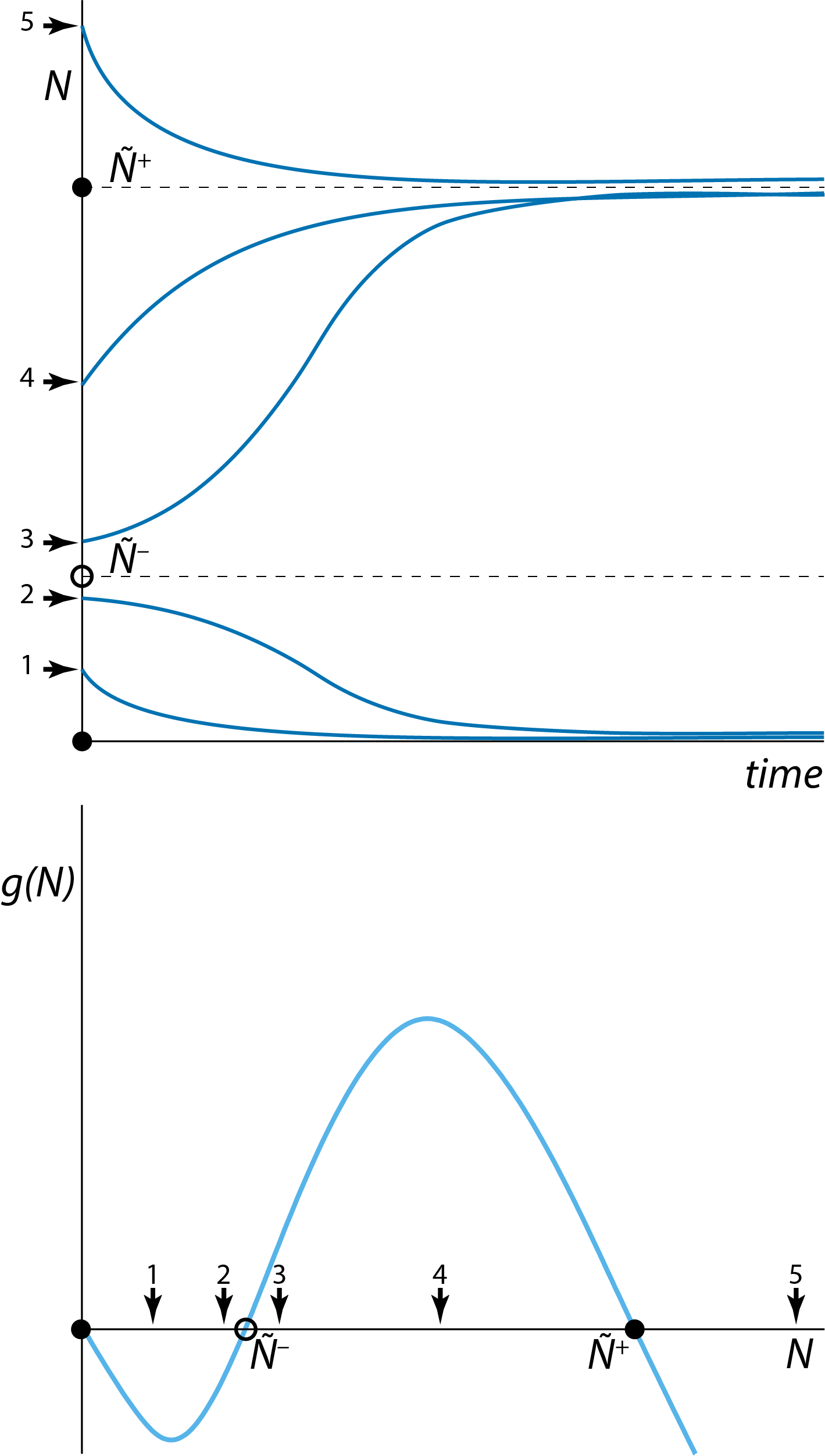
Figure 2.2: Five possible starting values of population abundance \(N(0)\) (arrows in bottom panel) and the qualitative shape of the dynamics resulting from these five different starting points (top) constructed on the basis of the graph relating the right-hand side \(g(N)\) to the population abundance \(N\) (bottom) for the two-sexes population model.
2.3 Bifurcation graphs: Parameter dependence of steady states
Step 1 in a mathematical analysis of a population dynamic model is to determine its steady states by figuring out for which values of the population abundance(s) \(N\) the right-hand side of the ODE, \(g(N)\), vanishes: \[\begin{equation} g(N) = 0 \end{equation}\] Doing some basic analysis on the function \(g(N)\) in equation (2.2) for the two-sexes population model, leads to the following 3 steady state values for the population abundance \(N\):
\[\begin{equation} \tag{2.4} \tilde{N}\;=\;0\\ \end{equation}\] \[\begin{equation} \tag{2.5} \tilde{N}\;=\;\tilde{N}^{-}\;=\;\dfrac{1}{2}\,\Gamma\,\left(1\:-\:\sqrt{1\,-\,4\dfrac{\delta}{\beta\Gamma}}\right) \end{equation}\] \[\begin{equation} \tag{2.6} \tilde{N}\;=\;\tilde{N}^{+}\;=\;\dfrac{1}{2}\,\Gamma\,\left(1\:+\:\sqrt{1\,-\,4\dfrac{\delta}{\beta\Gamma}}\right) \end{equation}\]
Because from now on I will be discussing steady state value of the two-sexes model I will consistently write \(\tilde{N}\) as opposed to simply \(N\) to make explicit that the values of \(N\) discussed are steady state values.
The values of these 3 steady states, at least of the latter two, depend on the model parameters. This dependence of steady states on model parameters can be graphically shown in a figure with on the x-axis a particular model parameter and on the y-axis the value of the steady state(s) of the model, indicated with \(\tilde{N}\). Such a figure is referred to as a bifurcation graph. Figure 2.3 shows this bifurcation graph of the two-sexes population model as a function of the model parameter \(\beta\).
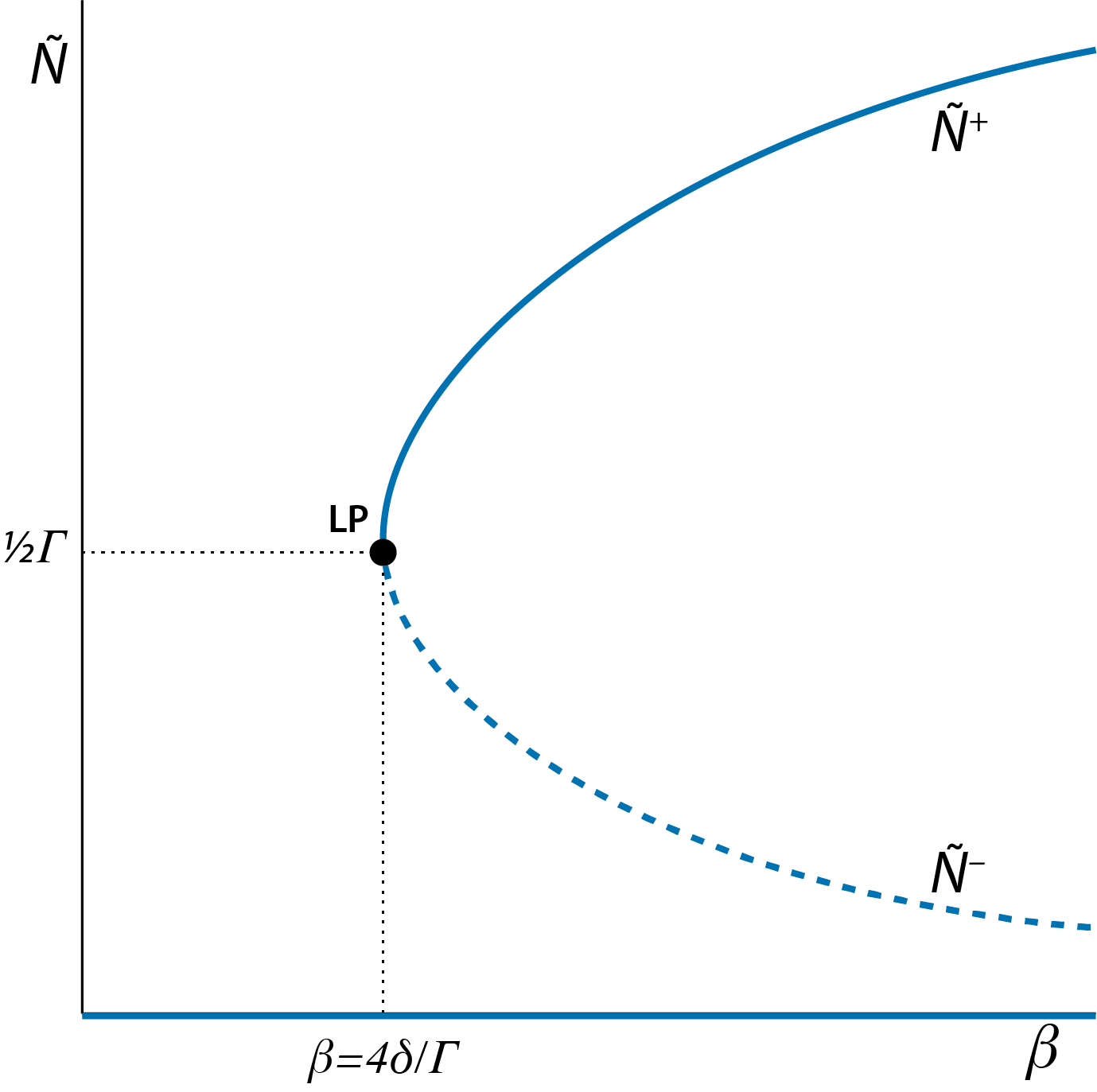
Figure 2.3: Bifurcation graph of the tow-sexes population model, showing the dependence of the steady state values \(\tilde{N}\) of the model as a function of the model parameter \(\beta\). Curve sections representing unstable steady states (saddle points) are indicated with dashed lines, curve sections representing stable steady states are indicated with solid lines. The special point indicated with ‘LP’, occurring at \(\beta=4\delta/\Gamma\) with \(\tilde{N}=\tfrac{1}{2}\Gamma\) is the limit point or saddle-node bifurcation point.
Figure 2.3 shows the location of one very special point, labeled ‘LP’: this is the point where the stable steady state occurring at \(\tilde{N}=\tilde{N}^{+}\) coincides with the unstable steady state occurring at \(\tilde{N}=\tilde{N}^{-}\). From the expressions for \(\tilde{N}^{-}\) and \(\tilde{N}^{+}\) given in equations (2.5) and (2.6), respectively, it can be inferred that this happens, when: \[ \sqrt{1\,-\,4\dfrac{\delta}{\beta\Gamma}} = 0 \] which occurs when \[\begin{equation} \beta=\dfrac{4\delta}{\Gamma} \tag{2.7} \end{equation}\] and consequently \[\begin{equation} \tilde{N}^{-}=\tilde{N}^{+}=\dfrac{1}{2}\Gamma \tag{2.8} \end{equation}\]
This special point labeled ‘LP’ in figure 2.3 is an important point because the value of \(\beta\) at which this limit point occurs indicates a threshold value at which the dynamics of the system shows a drastic, qualitative change: for \(\beta\) values below (to the left of) the limit point only a single steady state is possible \(\tilde{N}=0\). For values of \(\beta\) above (to the right of) the limit point 3 steady states occur: \(\tilde{N}=0\), \(\tilde{N}=\tilde{N}^{-}\) and \(\tilde{N}=\tilde{N}^{+}\).
Because of this major qualitative change in dynamics the point labeled ‘LP’ in figure 2.3 is called a bifurcation point. More specifically, this point is referred to as limit point or saddle-node bifurcation point. The term ‘limit point’, from which the abbreviation ‘LP” is derived, refers to the fact that the \(\beta\) coordinate of the point represents a limit that separates values of \(\beta\) that give rise to either 1 or 3 steady states. The term ’saddle-node bifurcation point’ refers to the fact that at this point a stable steady state, which is also referred to as a node, coincides and merges with an unstable steady state, a saddle point.
The limit or saddle-node bifurcation point shown in figure 2.3 is a very generic feature that can occur in any dynamical system of arbitrary complexity. Limit or saddle-node bifurcation points are important dynamical features as they are indicative of the occurrence of alternate stable states, the fact that over a range of conditions (i.e. model parameter values) a dynamical system has more than one stable equilibrium state. Furthermore, limit or saddle-node bifurcation points represent one of the most important mechanism underlying the occurrence of tipping points, which can be defined as a specific point at which a small change in conditions gives rise to a disproportionately large change in system dynamics. At the limit point shown in figure 2.3, for example, a small decrease in \(\beta\) from just above to just below the threshold value of \(\beta\) associated with the limit point may shift the equilibrium population abundance form \(\tilde{N}=\tilde{N}^{+}\) to \(\tilde{N}=0\).
Alternate stable states (also referred to as alternative stable states) and the tipping points associated with them have been shown or argued to occur in a wide variety of systems, ranging from freshwater lakes that are either dominated by algae or by underwater vegetation, to savanna-forest systems that are either controlled by herbivore grazing or by fire (see figure 2.4) and to the financial crises of 2008 when banks collapsed. Limit or saddle-node bifurcation points are therefore an important and generic feature of dynamical systems that every student of living systems should know about.
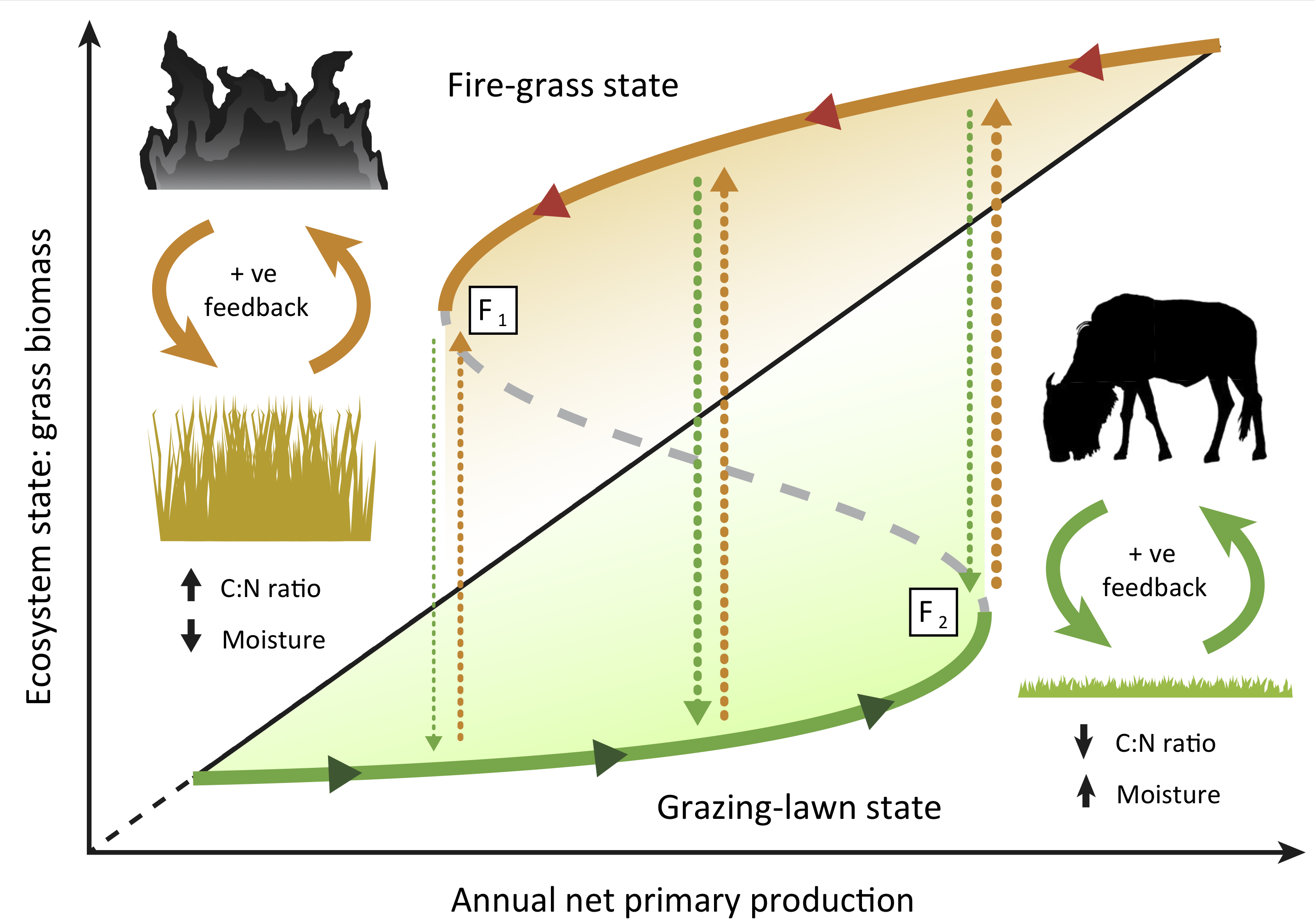
Figure 2.4: Figure I in Box I from Hempson et al. (2019) illustrating catastrophic shifts between alternate stable states in grassland communities. Conceptual diagram of alternate fire-grass (orange unbroken line) and grazing-lawn (green unbroken line) stable states along a productivity gradient. Each state is stabilized by positive feedbacks (filled orange and green arrows) with fire and grazers, respectively, a dynamic underpinned by opposing C:N ratios and leaf moisture traits amongst others. Transitions between states (broken lines) occur when shifts in rainfall exceed critical bifurcation points at \(F_1\) or \(F_2\), or when external factors precipitate changes. Shading represents grasses with higher palatability (green) or flammability (orange), respectively. The black diagonal line represents the general linear increase in grass biomass with annual net primary production.
2.4 Two-parameter graphs of different dynamical regimes
Figure 2.3 shows two distinct dynamic regime occurring for different ranges of the model parameter \(\beta\): a dynamic regime with only \(\tilde{N}=0\) as stable steady state of the population dynamics and a regime with \(\tilde{N}=0\) and \(\tilde{N}=\tilde{N}^{+}\) as stable steady states of the population dynamics (separated by the unstable steady state or saddle point \(\tilde{N}=\tilde{N}^{-}\)). To get an overview of the occurrence of these 2 different dynamical regimes at an even higher level of abstraction we can construct a figure with on each of the axis a separate model parameter and indicating for which combinations of parameter values the different dynamical regimes occur. Figure 2.5 illustrate such a two-parameter graph of dynamical regimes, as a function of the model parameters \(\beta\) and \(\Gamma\). The curve shown in figure 2.5 is given by the relation: \[ \Gamma = \dfrac{4\delta}{\beta} \]
which is derived from the expression for the critical value of \(\beta\) at the limit point (see equation (2.7)).
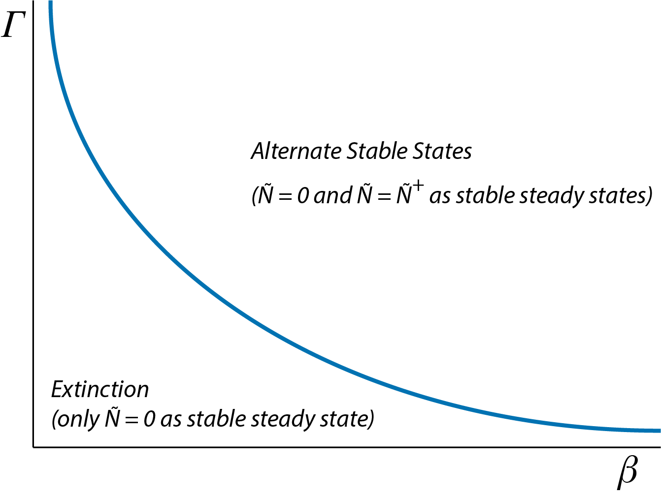
Figure 2.5: Two-parameter graph of dynamical regimes for the two-sexes population model, showing the combinations of parameter values for \(\beta\) and \(\Gamma\) for which either extinction occurs (\(\tilde{N}=0\) is the only stable steady state of the population dynamics) or alternate steady states occur (both \(\tilde{N}=0\) and \(\tilde{N}=\tilde{N}^{+}\) are stable steady states of the population dynamics).
2.5 Connecting phaseplane, timeseries, bifurcation and two-parameter graphs
A good grasp of the dynamics of a particular system requires that we understand how the different graphs, shown in the figures 2.1, 2.2, 2.3 and 2.5, are related to each other. The figure below shows these 4 graphs once again, including the connections between them.
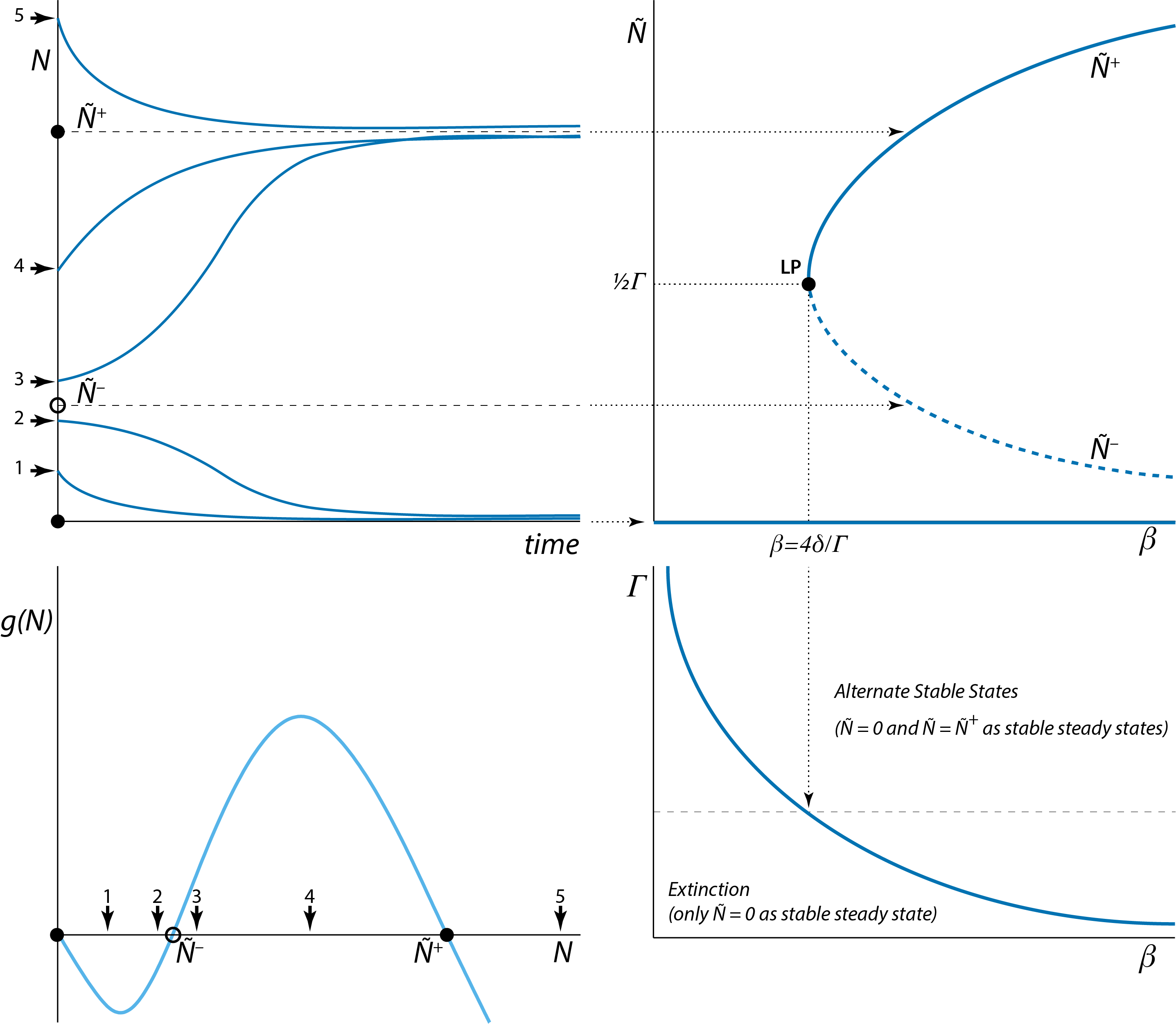
Figure 2.6: Top-left: Time series of dynamics of the two-sexes population model from the 5 different starting positions that are also shown in the graph of the population growth rate \(g(N)\) as a function of \(N\) (bottom-left). Top-right: The stable steady states \(\tilde{N}=0\) \(\tilde{N}=\tilde{N}^{+}\) indicated in the top-left and bottom-left graphs correspond to single points on the horizontal and curved solid lines, respectively, in the top-right graph, which shows the equilibrium abundance \(\tilde{N}\) as a function of \(\beta\). Similarly, the unstable steady state \(\tilde{N}=\tilde{N}^{-}\) corresponds to a single point on the curved dashed line in this graph. Bottom-right: The limit point shown in the top-right graph corresponds to a single point on the curve in the two-parameter graph that shows the boundary between the two different dynamical regimes.
Figure 2.2 already highlighted the connections between the graph of the population growth rate \(g(N)\) as a function of \(N\) and the qualitative shape of the curves representing the time series of population dynamics from different initial values \(N(0)\). The graphs of the population growth rate \(g(N)\) as a function of \(N\) and of the timeseries of dynamics from different initial values \(N(0)\), however, are always for a single combination of parameter values and do not reveal how dynamics change with parameter changes. The stable and unstable steady states identified in these graphs therefore correspond to single points on the curves in the bifurcation graph relating the equilibrium abundance \(\tilde{N}\) to the parameter \(\beta\) (figure 2.3 and top-right panel of figure 2.6). Likewise, the limit point identified in the bifurcation graph relating the equilibrium abundance \(\tilde{N}\) to the parameter \(\beta\) (figure 2.3 and top-right panel of figure 2.6) corresponds to a single point on the boundary curve shown in figure 2.5 and bottom-right panel of figure 2.6 that separates the dynamic regimes of extinction from the dynamic regime with alternate stable states.
A key aspect of these connections between the different graphs is that once a two-parameter graph of dynamical regimes as shown in figure 2.5 and bottom-right panel of figure 2.6 is given, it is possible to reconstruct from there the bifurcation graphs as a function of a single model parameters, since the bifurcation graph correspond to cross-sections through the two-parameter dynamical regime graphs in either the horizontal or the vertical direction. For example, the bifurcation graph in the top-left panel of figure 2.6 corresponds to a cross-section in the bottom-right panel of figure 2.6 at the particular value of \(\Gamma\) indicated with a horizontal thin dashed line in the latter panel. Two-parameter graphs of dynamical regimes as shown in the bottom panel of figure 2.6, which in some fields are referred to as operating diagrams, are frequently shown in publications and the capacity to relate these graphs to bifurcation graphs such as shown in the top-right panel of figure 2.6 is important for their interpretation.
Exercise: Based on the bottom-right panel of figure 2.6 one can now also quite easily generate a qualitative sketch of the bifurcation graph of \(\tilde{N}\) as a function of \(\Gamma\). Furthermore, given the expression for the limit point value (equation (2.7)) is should also be straightforward to sketch a two-parameter graph of the different dynamical regimes as a function of \(\beta\) and \(\delta\) and based on that a qualitative sketch of the bifurcation graph of \(\tilde{N}\) as a function of \(\delta\).
2.6 Mathematical analysis of steady state stability
Here I discuss what is usually the core part of the analysis of a population dynamic model. At the same time it is also mathematically the most demanding part of the analysis. The key problem is that the graphical analysis of model steady states discussed in section 2.1 is very useful for models consisting of one or two ODES, but is hardly usable for models of higher dimensions. In general, in more complicated situations the graphical method of analysis is very difficult, if not impossible, to apply. The technique discussed in this section constitute a more rigorous and robust method of analysis with the same aim as the graphical method of analysis: determining the qualitative behavior of the population dynamic model. More specifically, to determine whether steady states are (locally) stable or unstable, i.e. analyzing whether the population abundance would return to the steady state, if displaced away from it by a (infinitesimally) small, but otherwise arbitrary amount. This is achieved by means of a mathematically more rigorous approach that can also be applied in more complicated cases, for example, when the dynamics is described by 3 or even more ODEs.
To analyze the stability of the steady states, such as presented in equations (2.4), (2.5) and (2.6), we make use of two crucial mathematical properties:
Linear ODEs and even systems of linear ODEs can be solved explicitly
Every mathematical function \(g(N)\) can be approximated in a small neighborhood around a particular value \(N=\tilde{N}\) by its Taylor expansion: \[\begin{equation} \tag{2.9} g(N)\,=\,g(\tilde{N})\,+\,g^\prime(\tilde{N})\Delta_N\,+\, \dfrac{1}{2}g^{\prime\prime}(\tilde{N})\Delta_N^2\,+\, O\left(\Delta_N^3\right) \end{equation}\] in which I have used \(\Delta_N\) as a shorthand notation for: \[ \Delta_N := N-\tilde{N} \] An easy approximation of the function \(g(N)\) is obtained by dropping all terms that incorporate the quantity \(\Delta_N\) with a power of 2 or higher: \[\begin{equation} \tag{2.10} g(N)\,\approx\,g(\tilde{N})\,+\,g^\prime(\tilde{N})\Delta_N \end{equation}\] or written without the shorthand notation \(\Delta_N\): \[\begin{equation} \tag{2.11} g(N)\,\approx\,g(\tilde{N})\,+\,g^\prime(\tilde{N})\left(N-\tilde{N}\right) \end{equation}\] The right-hand side of this equation is referred to as the first-order Taylor approximation of the function \(g(N)\) in the neighborhood of \(N=\tilde{N}\). Note that the first-order Taylor approximation to the function \(g(N)\) in the neighborhood of \(N=\tilde{N}\) is a linear function of the population abundance \(N\), since both \(g(\tilde{N})\) and \(g^\prime(\tilde{N})\) have constant values.
In the section 2.1 the stability of a steady state was essentially determined by investigating whether the population state would return to the steady state after being displaced away from this steady state by an infinitesimally small amount. The displacement had to be very small to avoid ending up outside the basin of attraction of the steady state. Above I already used \(\Delta_N\) to indicate the difference between the actual density of the population \(N\) and its equilibrium density \(\tilde{N}\). Let’s now consider that this difference will be changing over time and hence write this small displacement away from the steady state as an explicit function of time \(\Delta_N(t)\): \[\begin{equation} \tag{2.12} \Delta_N(t) := N(t)\,-\,\tilde{N} \end{equation}\] The ODE \[\begin{equation} \tag{2.13} \dfrac{dN(t)}{dt}\,=\,g(N(t)) \end{equation}\] that represents our population dynamic model not only specifies the dynamics of the population abundance \(N(t)\), but because \(\Delta_N(t)\) is defined in terms of \(N(t)\) and a constant value \(\tilde{N}\), it also specifies the dynamics of this small displacement \(\Delta_N(t)\). Mathematically, this is expressed by the following: \[\begin{equation} \dfrac{d\Delta_N(t)}{dt}\,=\,\dfrac{d\left(N(t)-\tilde{N}\right)}{dt}\,=\, \dfrac{dN(t)}{dt}\,-\,\dfrac{d\tilde{N}}{dt}\,=\,\dfrac{dN(t)}{dt} \end{equation}\] Hence, the right-hand side of the ODE describing the dynamics of \(\Delta_N(t)\) is the same as the right-hand side of the ODE for \(N(t)\): \[\begin{equation} \dfrac{d\Delta_N(t)}{dt}\,=\,g(N(t)) \end{equation}\] Using the relation between \(\Delta_N(t)\) and \(N(t)\) in equation (2.12), this ODE can be rewritten as: \[\begin{equation} \dfrac{d\Delta_N(t)}{dt}\,=\,g(\tilde{N}+\Delta_N(t)) \end{equation}\] This last ODE still exactly describes the dynamics of the small displacement \(\Delta_N(t)\) away from the equilibrium \(\tilde{N}\). Moreover, as the function \(g(N)\) will generally be a non-linear function that is impossible to solve explicitly, also this exact ODE for the dynamics of \(\Delta_N(t)\) can not be solved explicitly. By rewriting the original ODE of the population model in terms of the dynamics of the small displacement \(\Delta_N(t)\) I have ended up with an ODE that is just as complicated and essentially I have not gained anything. However, using the fact that \(\Delta_N(t)\) is small I can gain a lot of analytic power, because it allows me to approximate the ODE (2.13) with an ODE in which I substitute the right-hand side \(g(\tilde{N}+\Delta_N(t))\) by its first-order Taylor expansion around \(\tilde{N}\): \[\begin{equation} \dfrac{d\Delta_N(t)}{dt}\,\approx\, g(\tilde{N})\,+\,g^\prime(\tilde{N})\Delta_N(t) \end{equation}\] Because \(\tilde{N}\) is an equilibrium, \(g(\tilde{N})\) equals 0. Hence, the ODE above simplifies to: \[\begin{equation} \tag{2.14} \dfrac{d\Delta_N(t)}{dt}\,=\,g^\prime(\tilde{N})\Delta_N(t) \end{equation}\] This final ODE is a linear one, which can be solved explicitly. Hence, the dynamics of \(\Delta_N(t)\) is given by: \[\begin{equation} \Delta_N(t)\;=\;\Delta_N(0)\,\exp\left(g^\prime(\tilde{N})\,t\right) \end{equation}\] in which \(\Delta_N(0)\) is the initial displacement away from the steady state \(\tilde{N}\). From this solution we can infer that the steady state is stable if the derivative of the function \(g(N)\) at the steady state value \(N=\tilde{N}\) is negative, while the steady state is unstable if this derivative is positive (When the derivative exactly equals 0 the steady state is at the edge of stability and instability and hence its stability is undetermined. This exceptional situation will not be discussed further here).
It should be noted that the relationship between the sign of the derivative of the function \(g(N)\) at the steady state value \(N=\tilde{N}\) and the stability of the steady state, was already discovered in section 2.1. There it was found that a steady state was stable if the slope of the curve \(g(N)\) as a function of \(N\) was negative, while the steady state was unstable if this slope was positive. Essentially, by deriving the linear ODE (2.14) for the small displacement \(\Delta_N(t)\) we have approximated the curve of \(g(N)\) as a function of \(N\) by a straight line through the point \(N=\tilde{N}\), i.e. by the tangent line in this point. The derivative of the function \(g(N)\) at \(N=\tilde{N}\) is exactly the slope of this tangent line and hence the slope of the curve \(g(N)\) as a function of \(N\). The approximation of the term \(g(\tilde{N}+\Delta_N)\) by its first-order Taylor expansion equal to \(g^\prime(\tilde{N})\Delta_N\) is therefore based on the assumption that in a very small neighborhood of the steady state \(N=\tilde{N}\) we can approximate the curve \(g(N)\) by its tangent line in \(N=\tilde{N}\), ignoring any higher order curvature.
The above process of deriving a linear ODE for the dynamics of a small displacement \(\Delta_N(t)\) in the neighborhood of a steady state \(N=\tilde{N}\) is referred to as local linearization of the dynamics, as the full model dynamics is locally represented by a linear type of dynamics. In mathematical literature the analysis is also referred to as linear stability analysis to indicate that the stability of a steady state is determined by a linear analysis.
The method discussed above for a model in terms of a single ODE is essentially the same as the method to determine the stability of a steady state in more complex models, for example models in terms of multiple ODEs. The analysis always consists of representing the model dynamics by its linear approximation in the neighborhood of a particular steady state to determine the fate of a small but arbitrary displacement (perturbation) away from the steady state. Once the linear approximation of the model in the neighborhood of an equilibrium is derived, a trial solution of the form \[\begin{equation} \tag{2.15} C e^{\lambda\,t} \end{equation}\] can be substituted into the linearized model equations (\(C\) is here some arbitrary constant). This approach will allow deriving an expression of the exponential rate(s) \(\lambda\) that are characteristic for the linearized dynamics in the neighborhood of the steady state. For a steady state to be stable all growth rates \(\lambda\) should be negative.
I will illustrate this procedure for the linearized ODE (2.14) even though its explicit solution has already been given. Substituting the trial solution (2.15) for \(\Delta_N(t)\) into the linearized ODE yields: \[\begin{equation} \dfrac{d C e^{\lambda\,t}}{dt}\,=\, g^\prime(\tilde{N}) C e^{\lambda\,t} \end{equation}\] The time derivative in the left-hand side of this ODE can be simplified to yield: \[\begin{equation} \lambda C e^{\lambda\,t}\,=\,g^\prime(\tilde{N}) C e^{\lambda\,t} \end{equation}\] After dividing both sides of the resulting equation by \(C\exp(\lambda t)\), the following equation is obtained: \[\begin{equation} \tag{2.16} \lambda\,=\,g^\prime(\tilde{N}) \end{equation}\] This equation is referred to as the characteristic equation, as it specifies the characteristic rate \(\lambda\) of the linearized dynamics. As was already concluded, if \(\lambda\) is positive the steady state is unstable, while it is stable if \(\lambda\) is negative. The quantity \(\lambda\), which you can interpret as a characteristic growth rate in case \(\lambda\) is positive and as a characteristic dampening rate if \(\lambda\) is negative, is in called the eigenvalue of the linearized dynamics.
The entire discussion of characteristic equation and eigenvalue in the context of the single ODE models that are the topic of this chapter is a little bit overdone. However, it illustrates nicely the approach taken with more complicated models, formulated in terms of systems of ODEs. In those cases, the characteristic equation is often a far more complicated equation which will only implicitly determine the eigenvalues. Surely, it will in general not be possible to specify the eigenvalues as explicitly as it is done in equation (2.16). Nonetheless, the idea is the same: a characteristic equation is derived for the linearized dynamics in the neighborhood of a steady state. This characteristic equation determines, usually in a rather difficult way, the eigenvalues (or characteristic growth rates) \(\lambda\), which all have to be negative for the particular steady state to be stable.
2.7 Early warning signals for tipping points and catastrophic shifts
The mathematical analysis of the stability of steady states discussed in the previous section yields one particular piece of information that was not apparent from the graphical analysis of the stability of a steady state presented in section 2.1: It reveals that small deviations from the equilibrium state \(N=\tilde{N}\) will change over time following \[ \Delta_N(t) = \Delta_N(0)e^{\lambda t} \] in which \(\Delta_N(0)\) is the initial perturbation away from the equilibrium. Any deviation will therefore die away or dampen at a characteristic rate \(\lambda\) (if \(\lambda < 0\)) or start to grow at a characteristic rate \(\lambda\) (if \(\lambda > 0\)). If we now consider the bifurcation graph shown in figure 2.3 for the steady state densities in the two-sexes population growth model as a function of the model parameter \(\beta\), we can conclude that for all the stable steady states (indicated with solid lines in figure 2.3) \(\lambda\) is negative, whereas for the unstable steady states (indicated with dashed lines in figure 2.3) \(\lambda\) is positive. At the limit point that occurs at \(\beta = 4\delta/\Gamma\), however, both the stable and unstable steady state coincide and merge, which necessarily implies that the values of \(\lambda\) that characterize these two merging steady states have to closer and closer to 0, the closer the value of \(\beta\) is to the critical value \(4\delta/\Gamma\) (remember that every steady state is characterized by its own, unique eigenvalue or set of eigenvalues in case of a more complex model). At the critical value \(\beta = 4\delta/\Gamma\) the stable and unstable steady state have merged into a single steady state with eigenvalue \(\lambda = 0\). Another way to see this is to draw the function \(g(N)\) characterizing the population growth rate in the two-sexes population model for the critical value \(\beta = 4\delta/\Gamma\). The expressions (2.5) and (2.6) for the unstable and stable steady state \(\tilde{N}^{-}\) and \(\tilde{N}^{+}\), respectively, show that these two steady state values coincide and are equal to \(\tfrac{1}{2}\Gamma\). The graph of \(g(N)\) for this critical value \(\beta = 4\delta/\Gamma\) is shown in the following figure:
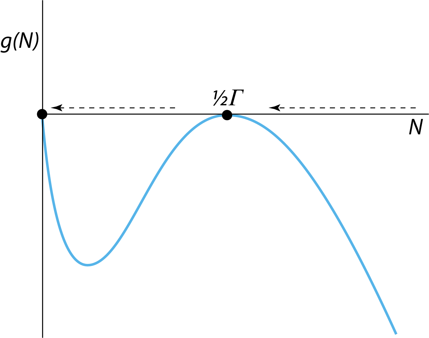
Figure 2.7: The right-hand side \(g(N)\) of the ODE describing the dynamics of the two-sexes population growth model for the critical value \(\beta=4\delta/\Gamma\). The horizontal arrows indicate that for values of \(N\) the population growth rate is negative (left-pointing arrows) and the population abundance \(N\) will therefore decrease over time, except for \(\tilde{N}=\tfrac{1}{2}\Gamma\).
From this figure it can be seen that the derivative \(g^\prime(\tilde{N})\) for \(\tilde{N}=\tfrac{1}{2}\Gamma\) equals 0 and hence \(\lambda = 0\).
The fact that the dampening rate \(\lambda\) of a stable steady state approaches 0, the closer a system is to a limit point or tipping point has been exploited to serve as an indicator whether or not the system is approaching a catastrophic collapse that is associated with the tipping point. The fact that the dampening rate approaches 0 implies that random perturbations to the system state die away more slowly the closer the system is to the tipping point. In the figure below it is illustrated that the brain activity of a person that experiences an epileptic seizure indeed shows an increasing variance, resulting from a decreasing dampening rate, in the minutes preceding the epileptic seizure.
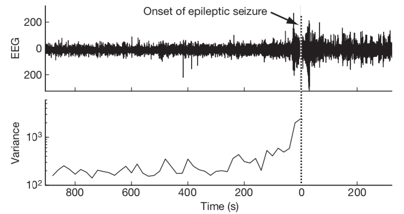
Figure 2.8: Subtle changes in brain activity before an epileptic seizure may be used as an early warning signal. The epileptic seizure clinically detected at time 0 is announced minutes earlier in an electroencephalography (EEG) time series by an increase in variance (Figure 5 from Scheffer et al. (2009)).
The epileptic seizure is hence postulated to be analogous to a saddle-node bifurcation point of the dynamical system that represents our brain functioning. The increasing variance in the timeseries, associated with the decreasing dampening rate and hence slower decay of random perturbations, has been used in a variety of systems as a so-called early warning signal for an upcoming catastrophic shift in the state of a system. A number of examples are discussed in the review by Scheffer et al. (2009).