Chapter 3 Transcritical bifurcation in an epidemic model

To discuss the characteristics of the second type of bifurcation point, a branching point or transcritical bifurcation point (remember the first, the second is jargon!), I will consider the epidemic spread of a disease in a population. In the middle of the Covid-19 epidemic this seems not only very appropriate, but it will also touch upon some by now famous technical concepts, like the R-value that is so often mentioned in newspapers.

Let’s consider a population of susceptible individuals, for which the population growth is described by the logistic growth equation. Denoting the abundance of the susceptible population with \(S\) the dynamics of \(S\) can then be described by:

\[ \dfrac{dS}{dt}=r S\left(1\:-\:\dfrac{S}{K}\right) \] in which the parameter \(K\) denotes the carrying capacity of the population and the parameter \(r\) denotes the population growth rate. The logistic growth of \(S\) implies that when started at low densities the abundance \(S\) of the susceptible population would follow a sigmoidal (S-shaped) curve as a function of time \(t\), approaching the carrying capacity \(K\) of the population. In the absence of any disease the only stable equilibrium state of the susceptible population is \[\begin{equation} \tag{3.1} \tilde{S} = K \end{equation}\] (\(S = 0\) is also an equilibrium state, but this equilibrium is unstable).

Now consider that a disease enters the population and let \(I\) denote the number of infected individuals in the population. Let’s furthermore assume that the disease can spread when an infected individual meets a susceptible individual. If we assume that infected and susceptible individuals mix homogeneously we can again use the ‘mass-action law’ (see section 2) and describe the infection rate with the term \[\begin{equation} \beta S I \end{equation}\] In this expression the parameter \(\beta\) represents a compound parameter that includes the probability that an infected and a susceptible individual meet each other, as well as the probability that when they meet the infected individual infects the the susceptible individual with the disease. To complete the model we have to make an assumption what happens with an individual after it gets infected. For simplicity I assume that an infected individual dies from the disease at a rate \(\delta\).

Note the assumption that an individual dies from the disease is dynamically equivalent to assuming that the individual recovers from the disease and is from then on immune to further infections. However, for simplicity and restrict the model to two variabels only I have assumed that only susceptible individual reproduce, which would not be a very realistic assumption when individuals would recover form the disease and acquite immunity.

3.1 The concept of the reproductive number \(R_0\)

The above contains all the assumptions to specify the complete population model. But before doing so, let’s explore the fate of an infected individual a little bit furthermore. I will use the variable \(P_i(\tau)\) to indicate the probability that an infected individual is still infectious (and alive) \(\tau\) time units after it became infected. This implies that at \(\tau=0\) \(P_i(0)=1\), as this refers to the moment the individual attracted the disease. The assumption that the infected individual dies from the disease at a rate \(\delta\) is a verbal representation of the mathematically less ambiguous assumption that \[\begin{equation} \dfrac{dP_i}{d\tau} = -\delta P_i(\tau) \end{equation}\] This linear ODE is straightforward to solve and yields together with the initial condition \(P_i(0)\) the solution: \[\begin{equation} \tag{3.2} P_i(\tau) = e^{-\delta \tau} \end{equation}\] To determine how long an infected individual on average remains infectious and can hence spread the disease we have to compute the integral over \(P_i(t)\) from \(\tau=0\) to \(\tau=\infty\): \[\begin{equation} \tag{3.3} \int_0^\infty P_i(\tau)\,d\tau = \int_0^\infty e^{-\delta \tau}\,d\tau = \dfrac{1}{\delta} \end{equation}\] Note that \(P_i(\tau)\) is a probability at the individual level and that hence the integral in the above equation represents the duration of the infectious period when averaged over a large number of individuals.

When the density of infected individuals is very small, an infected individual will only encounter susceptible individuals during the period it is infectious, at a rate that is proportional to the density of susceptible individuals, which then equals \(S\approx \tilde{S} = K\). The number of new infections that an infected individual will cause is therefore equal to: \[\begin{equation} \tag{3.4} R_0 = \dfrac{\beta K}{\delta} \end{equation}\] The quantity \(R_0\) is what in the news articles about Covid-19 is referred to as the \(R\)-number, except that the subscript 0 refers to the fact that it considers an infectious individual entering a completely susceptible population (\(\tilde{S}=K\)). The quantity \(R_0\) is a core element of theory about epidemics and plays a central role in the context of public health (Heesterbeek and Dietz 1996; Heesterbeek 2002).

3.2 Equilibrium states of the epidemic model

The full population model of the susceptible and infected part of the population can now be described by: \[\begin{align} \dfrac{dS}{dt}&=r S\left(1\:-\:\dfrac{S}{K}\right) - \beta S I \tag{3.5} \\ \dfrac{dI}{dt}&=\beta S I - \delta I \tag{3.6} \end{align}\] To derive an expression for the equilibrium state of the system with susceptible and infected individuals, the right-hand sides of both ODEs shown above have to be equated to 0 and solved simultaneously for appropriate values of \(S\) and \(I\). Consider when the right-hand side of the last ODE for \(dI/dt\) equals \(0\): \[ \beta S I - \delta I = 0 \] From this condition it can be inferred that it can only hold if either \(I=0\) or \(S=\delta/\beta\). When \(I=0\) the equilibrium value of \(S\) equals \(K\) as we derived above (see equation (3.1)). On the other hand, if in a dynamic equilibrium \(S=\delta/\beta\), the value of \(I\) should satisfy: \[ r \dfrac{\delta}{\beta} \left(1 - \dfrac{\delta}{\beta K}\right) - \beta \dfrac{\delta}{\beta} I \] The possible equilibrium states of the population model with susceptible and infected individuals are therefore the disease-free equilibrium, give by: \[\begin{equation} \begin{aligned} \tilde{S}&=K \\ \tilde{I}&=0 \end{aligned} \tag{3.7} \end{equation}\] and the endemic equilibrium, given by: \[\begin{equation} \begin{aligned} \tilde{S}&=\dfrac{\delta}{\beta} \\ \tilde{I}&=\dfrac{r}{\delta} \left(1 - \dfrac{\delta}{\beta K}\right) \end{aligned} \tag{3.8} \end{equation}\]

Now consider how these two possible equilibrium states of the model depend on model parameters. As an example we plot the values of the equilibrium states as a function of the model parameter \(\beta\), which represents the infectivity of the disease. This yields the following graph:

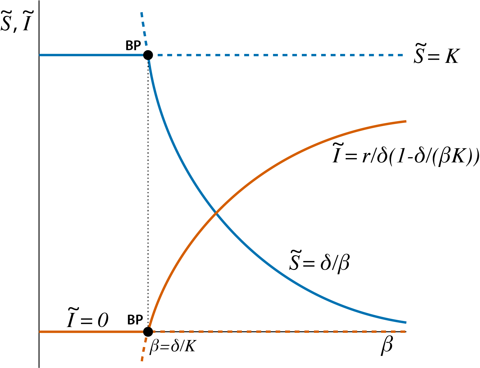
Figure 3.1: Bifurcation graph of the epidemic model, showing the steady state values \(\tilde{S}\) and \(\tilde{I}\) as a function of the model parameter \(\beta\). Curve sections representing unstable steady states (saddle points) are indicated with dashed lines, curve sections representing stable steady states are indicated with solid lines. The special point indicated with ‘BP’, occurring at \(\beta=\delta/K\) is the branching point or transcritical bifurcation point.

For low values of the infectivity parameter \(\beta\) the disease can not persist in the population because \[ \dfrac{\beta K}{\delta} < 1 \] which implies that the growth rate \(dI/dt\) is always negative (see equation (3.6)). As a consequence, the only possible equilibrium state is the disease-free equilibrium with \(\tilde{S}=K\) and \(\tilde{I}\). From a mathematical perspective the endemic equilibrium, given by (3.8), is still an equilibrium state of the model for such low values of \(\beta\), but because in this equilibrium \(\tilde{I}\) would be negative and \(\tilde{S}\) would be larger than \(K\) it is biologically irrelevant.

For values of \(\beta\) that are sufficiently high, such that \[ \tilde{S}=\delta/\beta < K \] the endemic state is a valid equilibrium of the epidemic model. Figure 3.1 shows that with increasing \(\beta\) values the density of susceptibles \(\tilde{S}\) in this endemic equilibrium decreases while the equilibrium density of infected individuals \(\tilde{I}\) increases.

The two equilibrium states represent two different curves as a function the model parameter \(\beta\). Of course, because figure 3.1 plots both the value of \(\tilde{S}\) as well as of \(\tilde{I}\), a total of 4 curves shows up in this figure, but for each model variable there are exactly two curves, corresponding to the two different equilibrium states. These two curves intersect at the point where \(\beta=\delta/K\), which implies that the equilibrium density of susceptibles \(\tilde{S}\) in the disease-free equilibrium (\(K\)) is exactly the same as the equilibrium density in the endemic equilibrium (\(\delta/\beta\)). The same holds for the density of infected individuals which equals 0 in both equilibrium states for \(\beta=\delta/K\). Figure 3.1 also shows smalls part of the curves corresponding to endemic equilibrium states with a negative density of infected individuals (\(\tilde{I}<0\)) and densities of susceptibles above the carrying capacity (\(\tilde{S}>K\)), even though these equilibrium states are biologically irrelevant. As mentioned before, mathematically these curve sections still represent valid equilibrium states of the model. They are included in figure 3.1 to illustrate that they are a natural extension of the curve parts that do represent biologically realistic states and to highlight that the branching point indicated with ‘BP’ in the figure is indeed an intersection point between two curves representing two different equilibrium states.

On biological grounds we can already argue that the stability of the equilibrium states changes at the branching point, as happens at every bifurcation point. For values \(\beta\) larger than \(\delta/K\) an infected individual entering a fully susceptible population with \(\tilde{S}=K\) will cause more than 1 new infection during the expected time that it is infectious (see equation (3.4)). Therefore, the disease-free equilibrium is unstable for \(\beta\) larger than \(\delta/K\) and the endemic equilibrium is the only stable steady state of the model. Therefore, if we consider increasing values of \(\beta\) the disease-free equilibrium changes from stable to unstable on crossing the threshold value \(\beta=\delta/K\), while at the same time the endemic equilibrium changes from unstable to stable. This is a generic phenomenon:

At branching points, in more technical terms also referred to as transcritical bifurcation points, two curves representing two different steady states of a dynamical system intersect and at the same time exchange their stability properties: the steady state that is stable at one particular side of the branching point is unstable at the other side, whereas the other steady state simultaneously and necessarily changes from unstable to stable.

In section 2.6 it was discussed how the stability of an equilibrium could be determined in a mathematically rigorous way. The same procedure could be used for the epidemic model as well, although it is more complicated as the model is formulated in terms of 2 ODEs as opposed to a single ODE. Nonetheless, the principal idea is the same: approximate the model in the neighborhood of an equilibrium state with a linear model (the local linearization of the model) by assuming that we only study very small deviations from this equilibrium state. After deriving the linearized equations for these small deviations from the equilibrium state, substitute an exponential trial solution of the form \[\begin{equation} \tag{3.9} C e^{\lambda\,t} \end{equation}\] and solve for the values of \(\lambda\) that would make this exponential function of time a valid solution of the linearized model. In the model discussed in section 2.6, which only contains a single ODE, a single such value of \(\lambda\) characterized the equilibrium state. Remember that each equilibrium state was characterized by its unique value of \(\lambda\), which in technical terms was referred to as eigenvalue. The more intuitive interpretation of the eigenvalue \(\lambda\) was that it characterized the rate at which small deviations from the equilibrium state would grow or die out over time.

For the epidemic model analyzed in this chapter only the outcome of this mathematical stability analysis will be presented, the details of the procedure will not be discussed. As a result, it is found that each steady state is characterized by two different eigenvalues, which is related to the fact that the model is formulated in terms of two model variables and hence the space representing all possible states that the model can attain is two-dimensional (This space of all possible states that a model can attain is also referred to as the phase space). Generically, a steady state of a dynamical system is characterized by as many eigenvalues as there are variables in the model. The disease-free steady state of the epidemic model is characterized by the following two eigenvalues (keep thinking about these eigenvalues as characteristic growth rates in the neighborhood of the steady state): \[\begin{align} \lambda_1&=-r \tag{3.10} \\ \lambda_2&=\beta K - \delta \tag{3.11} \end{align}\] These expressions show that \(\lambda_1\) is always negative, but \(\lambda_2\) is only negative as long as \(\beta K < \delta\). If \(\beta K > \delta\) \(\lambda_2\) is positive and a small deviation from the steady state will start to grow over time, moving the state of the system further and further away from the steady state. The transition where \(\lambda_2\) turns from negative to positive happens exactly at the branching point, where \(\beta = \delta/K\).

For completeness I also present here the expressions for the two eigenvalues that characterize the endemic steady state of the epidemic model: \[\begin{align} \lambda_1&=\;-\dfrac{1}{2}\dfrac{r\delta}{\beta K}\:-\: \dfrac{1}{2}\sqrt{\left(\dfrac{r\delta}{\beta K}\right)^2\,-\, 4r\delta\left(1-\dfrac{\delta}{\beta K}\right)} \tag{3.12} \\[2ex] \lambda_2&=\;-\dfrac{1}{2}\dfrac{r\delta}{\beta K}\:+\: \dfrac{1}{2}\sqrt{\left(\dfrac{r\delta}{\beta K}\right)^2\,-\, 4r\delta\left(1-\dfrac{\delta}{\beta K}\right)} \tag{3.13} \end{align}\] The expressions for these two eigenvalues are much more complicated, as they are derived from the general solution of a quadratic equation in terms of \(\lambda\). Since the first term in the expressions above is always positive (parameters in biological models are by definition positive quantities), only the value of \(\lambda_2\) can change sign when parameters change. The value of \(\lambda_2\) equals 0 when \[ \sqrt{\left(\dfrac{r\delta}{\beta K}\right)^2\,-\, 4r\delta\left(1-\dfrac{\delta}{\beta K}\right)} = \dfrac{r\delta}{\beta K} \] which happens when \[ 4r\delta\left(1-\dfrac{\delta}{\beta K}\right) = 0 \] Therefore, for the endemic steady state, in which \(\tilde{I}\) varies with parameters and is not always equal to 0 (as in the disease-free equilibrium), the value of the largest eigenvalue \(\lambda_2\) changes sign when \(\delta = \beta K\), which is once again the condition determining the branching point, where the disease-free and the endemic equilibrium coincide. This is the mathematical background for the change of stability of the two steady states that coincide at a branching point:

At branching points one of the eigenvalues of one of the two different, but coinciding steady states of the dynamical system changes from negative to positive, whereas one of the eigenvalues of the other steady state changes from positive to negative, such that the steady state that is stable at one particular side of the branching point is unstable at the other side, whereas the other steadfy state simultaneously and necessarily changes from unstable to stable.

3.3 Relating the bifurcation and dynamical regime graph

The branching point shown in figure 3.1 represents the boundary or threshold value that separates two distinct dynamical regimes: a regime in which the disease can not establish itself in the population and a regime in which the disease is continuously present in the population. As was also discussed in section 2.5 these different dynamical regimes can be summarized by constructing graphs as a function of two different model parameters with boundaries that separate parameter combinations with different dynamical outcomes from each other, as shown in figure 3.2.

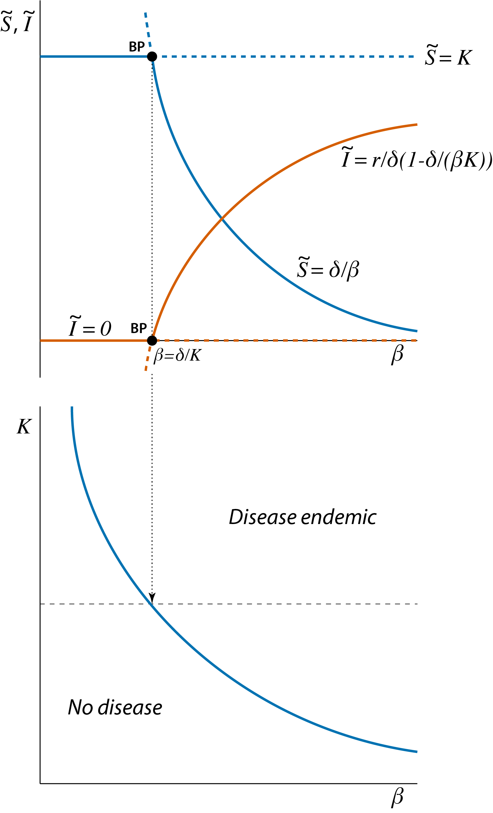
Figure 3.2: Relation between the bifurcation graph of the epidemic model (top panel, also shown in figure 3.1) and the two-parameter graph with different dynamical regimes of the model as a function of the model parameters \(\beta\) and \(K\) (bottom panel). The branching point shown in the top panel corresponds to a single point on the curve in the two-parameter graph that shows the boundary between the two different dynamical regimes.

The bifurcation graph shown in figure 3.1 is redrawn in the top panel of figure 3.2 to illustrate that it corresponds to a cross-section in the bottom panel of figure 3.2 at the particular value of \(K\) indicated with a horizontal thin dashed line. The bifurcation graph of a dynamical system as a function of a single model parameter and a dynamical regime graphs dependent on two model parameters are therefore tightly connected and can be translated into each other.