Chapter 4 Hopf bifurcation in a predator-prey model
To discuss the characteristics of the third type of bifurcation point, a Hopf bifurcation point, I will use as an example a well-known predator-prey model, described by the following system of ODEs:
\[\begin{align} \tag{4.1} \dfrac{dF}{dt}&=\;rF\left(1-\dfrac{F}{K}\right)\:-\: \dfrac{a F}{1\,+\,a h F}C\\[2ex] \tag{4.2} \dfrac{dC}{dt}&=\;\epsilon \dfrac{a F}{1\,+\,a h F}C\:-\:\mu C \end{align}\] In these ODEs the variables \(F\) and \(C\) refer to the prey and predator density, respectively. The first term in the right-hand side of equation (4.1) describing the prey dynamics: \[ rF\left(1-\dfrac{F}{K}\right) \] describes that in the absence of predators prey grow following the logistic growth equation with growth rate \(r\) and carrying capacity \(K\). The last term in the right-hand side of equation (4.1) describing the prey dynamics: \[ \dfrac{a F}{1\,+\,a h F}C \] describes that each predator forages on prey following a type II functional response \(aF/(1 + ahF)\) with attack rate \(a\) and handling time \(h\). This functional response originates in 0 for \(F=0\) and reaches an asymptote equal to \(1/h\) for very large values of \(F\) as predators under these conditions spend all their time handling the prey individuals they catch and do not loose any time searching for prey. Since predators need \(h\) time units to consume each prey they catch, the maximum number of prey they can possibly eat equals \(1/h\) per unit of time. The multiplication of the functional response with the density \(C\) shows that the total foraging rate of the predator population as a whole scales linearly with predator density and predators hence do not interfere with each other while foraging.
The first term in the right-hand side of equation (4.2) describing the predator dynamics: \[ \epsilon \dfrac{a F}{1\,+\,a h F}C \] shows that predators are assumed to produce new offspring at a rate that is proportional to their foraging rate with the parameter \(\epsilon\) representing the proportionality constant, which can also be interpreted as a conversion efficiency. Finally, the last term in the right-hand side of equation (4.2) describing the predator dynamics: \[ \mu C \] shows that predators are assumed to die at a constant death rate \(\mu\).
The predator-prey model presented above, which accounts for both logistic prey growth and a predator type II (or satiating) functional response, is also referred to as the Rosenzweig-MacArthur model after two authors that have investigated the dynamics of this model in great detail (Rosenzweig and MacArthur 1963; Rosenzweig 1971).
4.1 Dynamics of the Rosenzweig-MacArthur predator-prey model
To analyze the Rosenzweig-MacArthur, predator-prey model we can first look at the values of \(F\) and \(C\) for which either the prey density does not change and hence stays constant (that is, where \(dF/dt=0\)) or the predator density does not change and hence stays constant (that is, where \(dC/dt=0\)). The curves determined by the condition that \(dF/dt=0\) are called isoclines or nullclines of the prey dynamics, while the curves determined by the condition that \(dC/dt=0\) are called isoclines or nullclines of the predator dynamics. Equating the right-hand side of the ODE for the prey density (equation (4.1)) to 0, yields the following possible conditions for the prey nullclines: \[\begin{equation} \tag{4.3} F=0 \end{equation}\] \[\begin{equation} \tag{4.4} C=\dfrac{r}{a}\left(1-\dfrac{F}{K}\right)\left(1+a h F\right) \end{equation}\] Similarly, equating the right-hand side of the ODE for the predator density (equation (4.2)) to 0, yields the following possible conditions for the predator nullclines: \[\begin{equation} \tag{4.5} C=0 \end{equation}\] \[\begin{equation} \tag{4.6} F=\dfrac{\mu}{a (\epsilon -\mu h)} \end{equation}\]
Figure 4.1 shows the dynamics of the predator-prey model for different values of the prey carrying capacity \(K\) in the phaseplane of the model. The phaseplane is the plane spanned by the two variables in the model, the prey density \(F\) (plotted on the \(x\)-axis in figure 4.1) and the predatory density \(C\) (plotted on the \(y\)-axis in figure 4.1). For low values of the prey carrying capacity \(K\) the maximum density of prey (which is equal to \(K\)) is too low for the predators to persist. As can be inferred from the right-hand side of equation (4.2) describing the predator dynamics the per-capita growth rate of the predator (that is, the growth rate per predator individual) equals: \[ \epsilon \dfrac{a F}{1\,+\,a h F} - \mu \] and if \(K\) is very low this growth rate is smaller than 0: \[ \epsilon \dfrac{a K}{1\,+\,a h K} - \mu < 0 \] As a consequence, the only stable steady state of the model is an equilibrium without predators (\(\tilde{C}=0\)) and with prey density equal to the carrying capacity (\(\tilde{F}=K\)). The top-left panel in figure 4.1 illustrates these dynamics.
For larger values of \(K\) the predator per-capita growth rate is positive: \[ \epsilon \dfrac{a K}{1\,+\,a h K} - \mu > 0 \] and predators can grow from low density and persist. The result is a stable equilibrium state with prey and predators, as shown in the top-right panel of figure 4.1.
For even larger values of \(K\) the steady state with positive prey and predator density is no longer approached in a smooth way, but prey and predator density fluctuate around their equilibrium densities before asymptotically approaching these (see the bottom-left panel of figure 4.1). This dynamics is referred to as damped oscillations. The equilibrium is still stable, but the state of the system spirals around the equilibrium point on its approach toward the equilibrium values. The steady state is hence also referred to as a stable spiral.
Finally, for even larger value of \(K\) the steady state looses its stability altogether, as shown in the bottom-right panel of figure 4.1. When the equilibrium looses its stability a limit cycle emerges. A limit cycle is a closed, invariant loop in the state space (the black closed curve in the bottom-right panel of figure 4.1) which the state of the system approaches over time. This means that if an initial point is chosen right on the limit cycle, the state of the system will move along the limit cycle for all time. When the initial densities of prey and predator are somewhere outside this limit cycle, the dynamics will spiral inward and asymptotically approach the closed curve. In contrast, when the initial densities of prey and predator are somewhere close to the unstable equilibrium point inside the limit cycle, the dynamics will spiral outward and asymptotically approach the limit cycle. The bottom-right panel of figure 4.1 also illustrates these two different types of dynamics. In terms of dynamics over time, the limit cycle implies that population abundances will fluctuate.
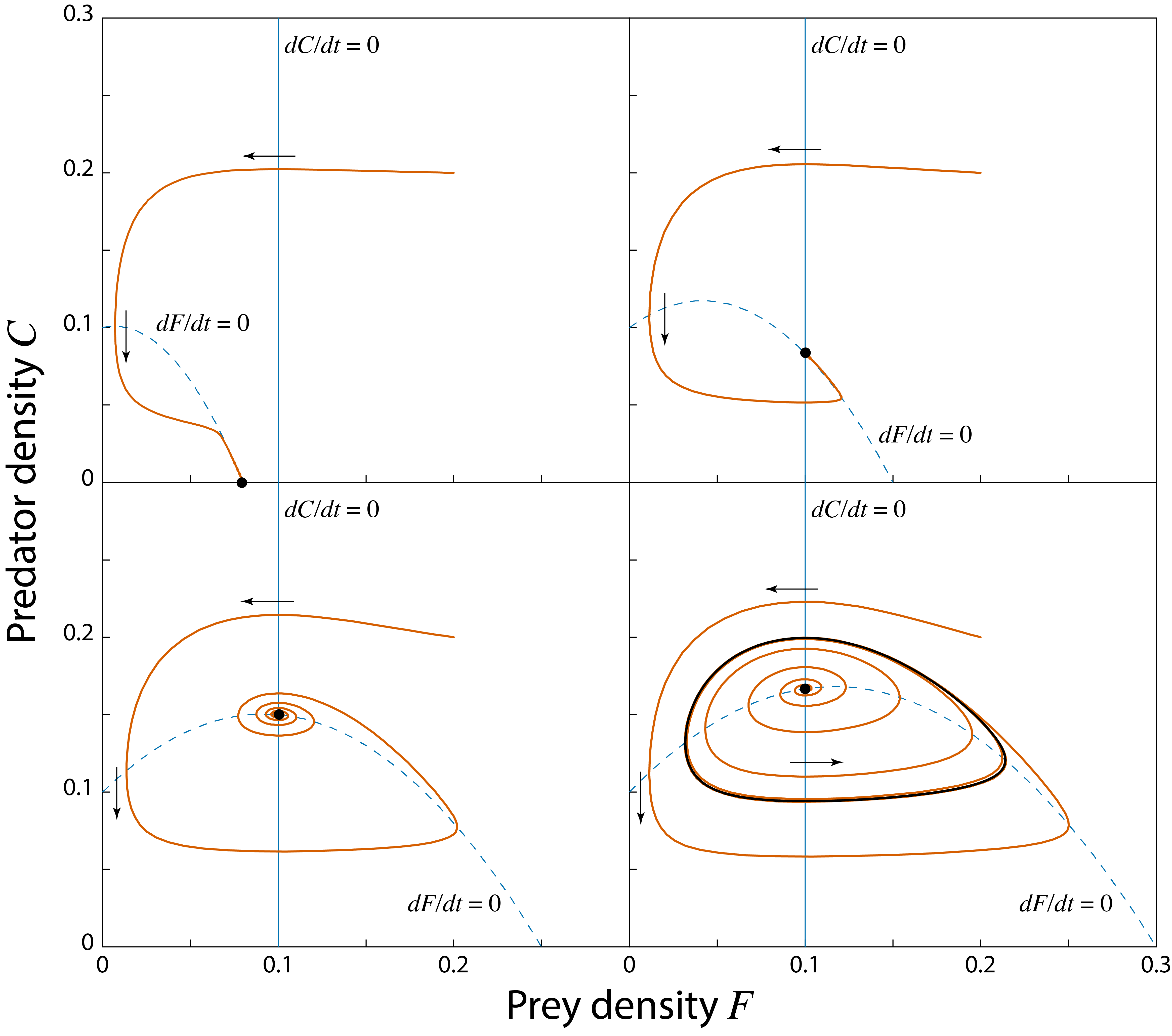
Figure 4.1: Solution curves in the phase plane of the Rosenzweig-MacArthur predator-prey model. Two isoclines where \(dF/dt=0\) (vertical, thin solid line) and \(dC/dt=0\) (hump-shaped, thin dashed line) are drawn (the isoclines coinciding with the \(x\)- and \(y\)-axis have been omitted). The isoclines intersect in the internal steady state. Top-left panel: \(K=0.08\); the internal steady state is biologically irrelevant, the prey-only equilibrium is a stable equilibrium. Top-right panel: \(K=0.15\); the internal steady state is a stable equilibrium. Bottom-left panel: \(K=0.25\); the internal steady state is a stable spiral. Bottom-right panel: \(K=0.3\); the internal steady state is an unstable spiral. In this latter figure two trajectories are drawn: one starting close to the unstable steady state, the other starting far away from it. Both approach the unique limit cycle (thick solid line). Other parameter values: \(r=0.5\), \(a=5.0\), \(h=3.0\), \(\epsilon=0.5\) and \(\mu=0.1\).
4.2 Bifurcation graph as function of prey carrying capacity \(K\)
The qualitative transitions occurring in the Rosenzweig-MacArthur predator-prey model can be shown most clearly by constructing a 3-dimensional graph with prey and predator density as a function of \(K\), as shown in figure 4.2. Two different bifurcation points occur: at low values of \(K\) a threshold occurs separating the values of \(K\) for which predators go extinct from those \(K\) values for which they can persist. From the previous section it should be clear that this threshold represents a branching point or transcritical bifurcation point. In figure 4.2 this threshold value is indicated with \(K_1\). The branching point that occurs at this threshold shows the typical configuration that was also shown in figure 3.1, in which a curve representing steady states with a zero density (in this case zero predator density; the straight solid and dashed line in the bottom plane of figure 4.2) intersects with a second curve representing steady states with non-zero densities (for both prey and predator in this case; the solid and dashed curve extending into the interior of the 3-dimensional space in figure 4.2). At the branching point the two different steady states coincide and the stability properties of both change simultaneously: the prey-only equilibrium changing from stable to unstable, while the prey-predator steady state changes from unstable to stable (refer to the discussion of figure 3.1).
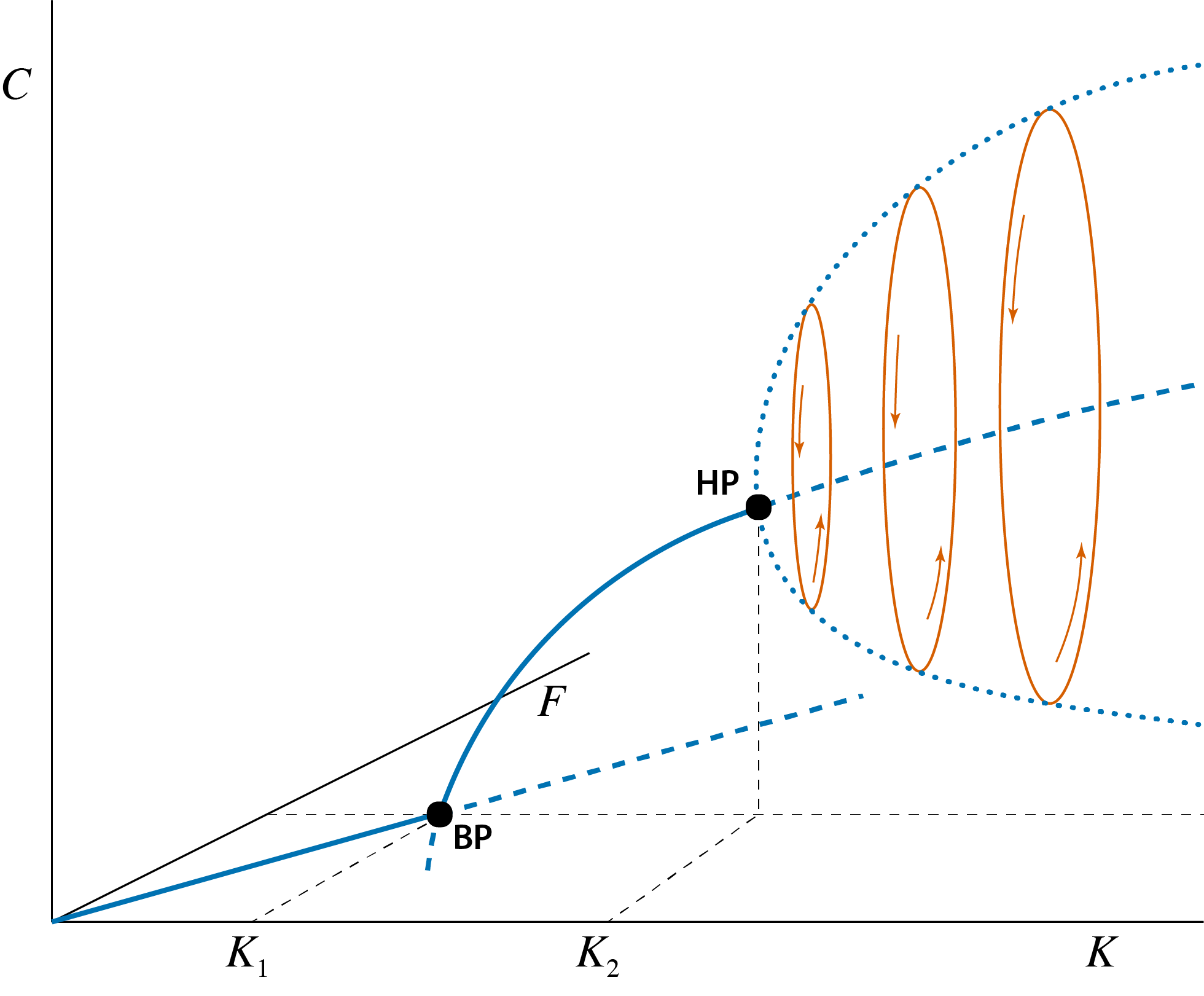
Figure 4.2: Bifurcation graph of the predator-prey model, showing the steady state values of prey \(\tilde{F}\) and predator \(\tilde{C}\) as a function of the model parameter \(K\) representing the prey carrying capacity. Curve sections representing unstable steady states are indicated with dashed lines, curve sections representing stable steady states are indicated with solid lines. The special point indicated with ‘BP’, occurring at \(K=K_1\) is the branching point or transcritical bifurcation point, above which predators can persist. The special point indicated with ‘HP’ occurring at \(K=K_2\) is the Hopf bifurcation point at which the predator-prey equilibrium changes form stable to unstable and a limit cycle emerges. With increasing values of \(K\) these limit cycles increase in amplitude. The thick dotted line indicates the amplitude of these cycles in the predator abundance. The three ellipse-shaped closed curves illustrate this limit cycle in both prey and predator density with thin arrows inidcating the direction of rotation.
The transition of the steady state with positive densities of both prey and predator from stable to unstable occurs in what is called a Hopf bifurcation point. As explained in the previous section at larger values of \(K\) the prey-predator equilibrium looses its stability while at the same time a limit cycle emerges, that is a closed loop of prey and predator densities which all timeseries of dynamics of the model tend to approach. For a number of different values of \(K\) the limit cycle is also indicated in this figure. Initially, in the Hopf bifurcation point the amplitude of this limit cycle is very small (in essence, infinitesimally small or zero amplitude), but the amplitude of this limit cycle grows quickly with increasing prey carrying capacity \(K\). The (infinite) collection of limit cycles for all parameter values \(K\) constitutes a parabolic object in the 3-dimensional space. In figure 4.2 this growing amplitude is illustrated by a curve that for each value of \(K\) plots the minimum and the maximum value of prey density attained during the limit cycle (thick dotted line in figure 4.2).
Analogous to what was discussed in sections 2.6 and 3.2 the changes in stability of the steady states in the predator-prey model analyzed here are governed by eigenvalues that intuitively can be understood as the rate at which small deviations from the equilibrium state would grow or die out over time. In section 3.2 it was discussed that each steady state of the epidemic model was characterized by two such eigenvalues, since the model was formulated in terms of two variables. The same holds for the predator-prey model discussed here: it is formulated in terms of two variables \(F\) and \(C\) and the dynamics in a small neighborhood of each steady state is governed by two eigenvalues. To compute these eigenvalues a procedure has to be followed that is similar to what is discussed in section 2.6: approximate the model in the neighborhood of an equilibrium state with a linear model (the local linearization of the model) by assuming that we only study very small deviations from this equilibrium state. After deriving the linearized equations for these small deviations from the equilibrium state, substitute an exponential trial solution of the form \[\begin{equation} \tag{4.7} C e^{\lambda\,t} \end{equation}\] and solve for the values of \(\lambda\) that would make this exponential function of time a valid solution of the linearized model.
As for the epidemic model analyzed in section 3.2 also for the predator-prey model is the mathematical derivation of expressions for these eigenvalues, which are usually indicated with the symbol \(\lambda\), beyond the scope of this introduction. In fact, the expressions for the eigenvalues \(\lambda\) in terms of the model parameters are so complicated that they are only give for completeness in the following note:
For the mathematically interested reader only
The two eigenvalues pertaining to the steady state of the predator-prey model with positive densities of both prey and predator equal the following expression of the model parameters: \[\begin{align} \lambda_1&=\;\dfrac{1}{2}\:r\,\left(\dfrac{\mu\,h}{\epsilon}\,+\, \dfrac{\mu}{\epsilon a K}\,-\, 2\,\dfrac{\mu}{a K (\epsilon -\mu h)}\right) +\:\dfrac{1}{2}\sqrt{\delta}\\[3ex] \lambda_2&=\;\dfrac{1}{2}\:r\,\left(\dfrac{\mu\,h}{\epsilon}\,+\, \dfrac{\mu}{\epsilon a K}\,-\, 2\,\dfrac{\mu}{a K (\epsilon -\mu h)}\right) -\:\dfrac{1}{2}\sqrt{\delta} \end{align}\]
where the quantity \(\delta\) is defined as:
\[\begin{equation} \delta = r^2\,\left(\dfrac{\mu\,h}{\epsilon}\,+\, \dfrac{\mu}{\epsilon a K}\,-\, 2\,\dfrac{\mu}{a K (\epsilon -\mu h)}\right)^2\,-\, 4\dfrac{r\mu}{\epsilon}\, \left(\epsilon\,-\,\mu\,h\,-\,\dfrac{\mu}{a K}\right) \end{equation}\]The key point about the eigenvalues for the predator-prey steady state with positive densities for both prey and predator is that they are complex numbers. Complex numbers are likely not familiar to the majority of readers as it is not a standard part of high-school mathematics. The set of complex numbers can be viewed as an extension of the set of real numbers \(\mathbb{R}\) that everybody should be familiar with. The extension of this latter set is necessary to deal with numbers that involve the square root of a negative number, an operation that in the set of real numbers \(\mathbb{R}\) is not permissible. More specifically, the set of complex numbers includes as a basic element the square root of -1, which is always indicated with the symbol \(i\) and which is referred to as the imaginary number: \[ i=\sqrt{-1} \] Any complex number can now be written as a sum of a real part (that is a number from the set of real numbers \(\mathbb{R}\)) and an imaginary part, which is a multiple of this imaginary number \(i\). The imaginary part is therefore a product of this imaginary number \(i\) and a number from the set of real numbers \(\mathbb{R}\).
In the predator-prey model the eigenvalues characterizing the dynamics in the neighborhood of the predator-prey steady state with positive densities for both prey and predator are complex numbers as soon as the dynamics in the phaseplane of the model spiral around the steady state (see the bottom panels in figure 4.1). The eigenvalues are then of the form: \[\begin{equation} \tag{4.8} \lambda_1 = a + b i \end{equation}\] and \[\begin{equation} \tag{4.9} \lambda_2 = a - b i \end{equation}\] with the real part of both \(\lambda_1\) and \(\lambda_2\) equal to \(a\) and the imaginary part equal to \(+b\) and \(-b\), respectively, (of course times \(i\)). The plus and minus sign in the imaginary part of \(\lambda_1\) and \(\lambda_2\) is significant: indeed complex eigenvalues always occur in pairs with the same real part (\(a\)), while one eigenvalue has a positive imaginary part (\(+b\)) and the other has a negative imaginary part (\(-b\)). The multiplier \(b\) of the imaginary part in these eigenvalues determines the period of the fluctuations around the steady state, that is the speed with which the state of the system spirals around the steady state. The real part \(a\) of the eigenvalues determines whether deviations from the steady state grow or shrink over time. If \(a\) is negative such deviations die away over time, in which case the dynamics spiral toward the steady state. The steady state is then referred to as a stable spiral (see bottom-left panel in figure (see bottom-right panel in figure 4.1)). If \(a\) is positive deviations from the steady state grow over time. The dynamics exhibit a spiraling away from the steady state, which is referred to as an unstable spiral, and the system approaches the limit cycle (see bottom-right panel in figure 4.1). At the Hopf bifurcation point the real part \(a\) of the two eigenvalues \(\lambda_1\) and \(\lambda_2\) is equal to 0, turning from negative to positive when increasing the value of \(K\) from below the critical value \(K_2\) to above the critical value \(K_2\). A change in stability of the steady state is therefore as before associated with a change from negative to positive but now from the real part of the eigenvalues.
4.3 Relating the bifurcation and dynamical regime graph
The branching point shown in figure 4.2 represents the boundary or threshold value that separates two distinct dynamical regimes: a regime in which the predator can not establish itself in the population and a regime in which the predator persists. Similarly, the Hopf bifurcation point shown in figure 4.2 also represents the boundary or threshold value separating two distinct dynamical regimes: a regime in which prey and predator approach a stable equilibrium and a regime in which prey and predator densities show persistent fluctuations that do not dampen over time. As was also discussed in the section 2.5 and 3.3 these different dynamical regimes can be summarized by constructing graphs as a function of two different model parameters with boundaries that separate parameter combinations with different dynamical outcomes from each other, as shown in figure 4.3 as a function of the prey carrying capacity \(K\) (on the \(x\)-axis) and the predator mortality rate \(\mu\) (on the \(y\)-axis).
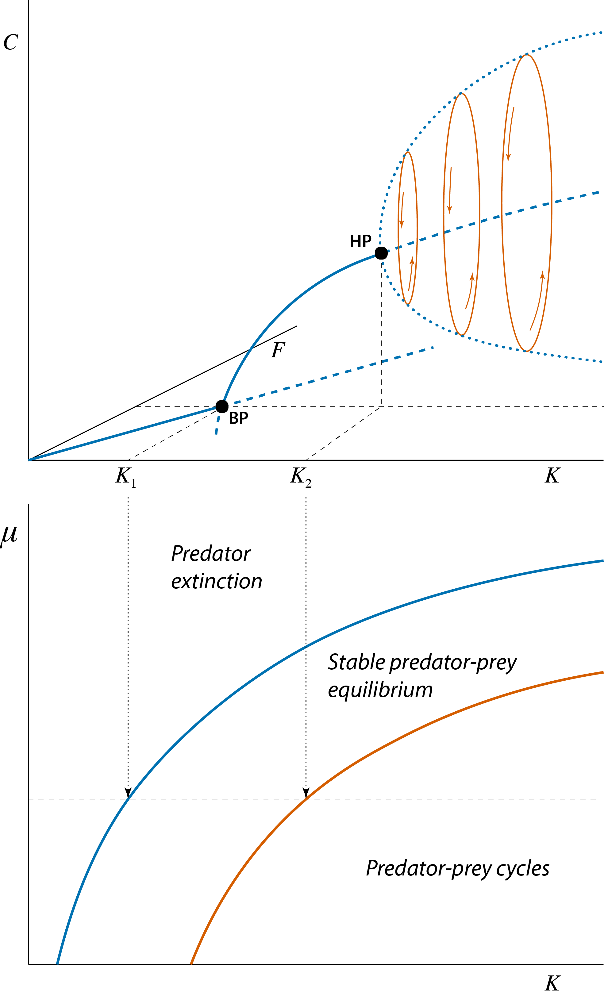
Figure 4.3: Bifurcation graph of the predator-prey model, showing the steady state values of prey \(\tilde{F}\) and predator \(\tilde{C}\) as a function of the model parameter \(K\) representing the prey carrying capacity. Curve sections representing unstable steady states are indicated with dashed lines, curve sections representing stable steady states are indicated with solid lines. The special point indicated with ‘BP’, occurring at \(K=K_1\) is the branching point or transcritical bifurcation point, above which predators can persist. The special point indicated with ‘HP’ occurring at \(K=K_2\) is the Hopf bifurcation point at which the predator-prey equilibrium changes form stable to unstable and a limit cycle emerges. With increasing values of \(K\) these limit cycles increase in amplitude. The thick dotted line indicates the amplitude of these cycles in the predator abundance. The three ellipse-shaped closed curves illustrate this limit cycle in both prey and predator density with thin arrows inidcating the direction of rotation.
The bifurcation graph shown in figure 4.2 is redrawn in the top panel of figure 4.3 to illustrate that it corresponds to a cross-section in the bottom panel of figure 4.3 at the particular value of \(\mu\) indicated with a horizontal thin dashed line. The bifurcation graph of a dynamical system as a function of a single model parameter and a dynamical regime graphs dependent on two model parameters are therefore tightly connected and can be translated into each other. The bifurcation graph in top panel of figure 4.3 shows two different bifurcation points, a branching point ‘BP’ and a Hopf bifurcation point ‘HP’, which correspond to single points on the two different boundary curves shown in the bottom panel of figure 4.3. The boundary curve that is associated with the branching point (top curve in the bottom panel of figure 4.3) separates all parameter combinations of prey carrying capacity \(K\) and predator mortality rate \(\mu\) that either lead to predator extinction (above the boundary curve) or to a stable predator-prey equilibrium (below the boundary curve). Analogously, the boundary curve that is associated with the Hopf bifurcation point (bottom curve in the bottom panel of figure 4.3) separates all parameter combinations of prey carrying capacity \(K\) and predator mortality rate \(\mu\) that either lead to a stable predator-prey equilibrium (above the boundary curve) or lead to persistent fluctuations in predator and prey density that do not dampen (below the boundary curve).