Chapter 5 Model analysis with deBif

In the computer labs we will use an R package called deBif that is specifically designed for the numerical analysis of (systems of) ordinary differential equations (ODEs). The package includes two basic functions, called deBif::phaseplane() and deBif::bifurcation(). The function phaseplane() allows for the numerical integration of (systems of) ODEs and for analysis of these ODEs in their phaseplane. In addition to numerical integration of ODEs the function bifurcation() allows for numerical bifurcation analysis of ODEs as a function of a single bifurcation parameter and for computing bifurcation curves as a function of two free parameters.

5.1 Installation of deBif

5.1.1 Installation of deBif as binary package from CRAN

To use the deBif package you will need a recent version of R as well as Rstudio and a range of additional R packages that are required.

Here are the necessary steps for the installation of R and Rstudio:

1. The version of Rstudio you use is not as critical as the version of R. Updating Rstudio is however easy and can be done via the following link:

   https://rstudio.com/products/rstudio/download/

2. The version of R you are using is critical. When you start up Rstudio you will see a welcome message in the pane of Rstudio that is called Console. The welcome message shows the version of R that you have installed. The version has to be at least 4.0. The package that we are going to use has been tested to work under R version 4.2.2 on Mac OS and version 4.0.3 on Windows. If you need to update your R installation, visit the following link:

   https://cran.r-project.org

The deBif package is available on CRAN (The Comprehensive R Archive Network). Therefore, once you have R and Rstudio installed you can most easily install deBif by choosing Tools->Install Packages in Rstudio and typing in the name. This will install deBif as well as the R packages that are needed to run the programs.

Once you have everything installed, you can load and test the package with the following 2 statements:

library(deBif)
deBifExample("rosenzweig")

5.1.2 Installation the most recent version of deBif

In case installation from CRAN fails or you want to install the most recent version of deBif from GitHub, the package has to be compiled and your R has to be tailored for that. Make sure that the appropriate versions of R and Rstudio have been installed as described in the previous section.

1. If you are working on Windows you will have to install both the base part of R as well as Rtools, which is needed to install packages that require compilation (you will need this for the package deBif). You can install Rtools from

   https://cran.r-project.org/bin/windows/Rtools/

   The recommended version of Rtools at the moment is Rtools42. The installation of Rtools takes some time.

2. Once you have the appropriate versions of Rstudio and R you first have to install the package devtools. You can do this by executing the command:

   install.packages("devtools", type = "binary")

   This command will download and install a range of R packages that are required by the devtools package, but should finish successfully. If you are asked to install these new packages, answer ‘yes’. In case you are asked to install from source and compile (this should not happen with the argument type = "binary"), answer ‘no’ to just install the compiled packages.

3. Once the package devtools is installed, the package deBif can be installed with the following command:

   devtools::install_github("amderoos/deBif")

   This will once again install additional packages that are required by the program. On my Windows my machine, after installing a new version of both Rstudio and R the devtools::install_github command failed with a message that ‘Git’ was not installed on my system. This was however solved by installing the package git2r, either via Tools -> Install packages or by executing the command install.packages("git2r", type = "binary").

4. Once you have everything installed, you can load and test the package with the following 2 statements:

   library(deBif)
   deBifExample("rosenzweig")

5.2 Model implementation

Before you begin with one of the following computer labs, first read how a system of ODEs has to be implemented in R to allow its analysis with either phaseplane() or bifurcation(). These two functions work with the same implementation of a system of ODEs. Section 1 of the manual for the deBif package describes in more detail how to implement the ODEs and how to use the functions phaseplane() and bifurcation(), although the graphical interface of these two function is rather intuitive and self-explanatory. You access the manual by executing in Rstudio the command:

deBifHelp()

The implementation of a model is identical to the implementation used in the package deSolve for systems of ODEs. The model implementation has 3 elements: a vector of state variables, a vector of parameters and the specification of the right-hand side of the ODEs. Both the vector of state variables and the vector of parameters, should consist of named vector elements only. The right-hand sides of the ODEs have to be specified in a R function with a name that you can choose yourself.

As an example, consider the logistic growth model:

\[\begin{align*} \dfrac{dN}{dt}&=\;r N \left(1- \dfrac{N}{K}\right) \end{align*}\]

with variable \(N\) representing the population density. The parameters in this model are the per-capita growth rate \(r\) and its carrying capacity \(K\).

To implement this model first a named vector of values for the state variables has to be defined:

state <- c(N = 0.01)

and similarly a named vector of default values for the parameters:

parms <- c(r = 0.1, K = 10.0)

The named elements of the state variable vector and the parameter vector can now be used in the function that described the right-hand side of the ODEs:

logistic <- function(t, state, parms) {
  with(as.list(c(state,parms)), {

    dNdt = r*N*(1 - N/K)

    return(list(c(dNdt)))
  })
}

To carry out bifurcation analysis of the logistic growth model implemented above an R script can be created with the following content:

# The initial state of the system has to be 
# specified as a named vector of state values.
state <- c(N = 0.01)

# Parameters has to be specified as a named vector of parameters.
parms <- c(r = 0.1, K = 1.0)

# The model has to be specified as a function that returns
# the derivatives as a list. You can adapt the body below
# to represent your model
logistic <- function(t, state, parms) {
  with(as.list(c(state,parms)), {

    dNdt = r*N*(1 - N/K)

    # The order of the derivatives in the returned list has to be
    # identical to the order of the state variables contained in
    # the argument `state`
    return(list(c(dNdt)))
  })
}

bifurcation(logistic, state, parms)

For more details see Section 1 of the manual for the deBif package.

5.3 Computer practical 1: Harvesting Cod

In 1497 the ocean around Newfoundland (Canada) was once so full of cod that explorer John Cabot marveled that they virtually blocked his ship. In 1992 the Canadian cod industry collapsed. Years of over-fishing had reduced the stock to dangerous levels, and the Canadian government was finally forced to put a stop to the drastic over-fishing. 40,000 people lost their jobs. In 2001 Cod stocks in the North Sea are down to one-tenth of the level 30 years ago. Scientists fear that North Sea cod may go the way of those in the Grand Banks of Canada, where over-fished stocks disappeared in 1992 and have not revived.

Consider the following differential equation:

\[ \dfrac{dN}{dt}\;=\;r\,N\,\left(1\:-\:\dfrac{N}{K}\right) \]

Here \(N\) stands for the Cod population (in 100.000 tons of cod), \(r\) is the intrinsic growth rate (per day), and \(K\) is the carrying capacity (in 100.000 tons of cod). This is the familiar logistic growth equation that describes the growth of most self-limiting populations. We are interested in describing the qualitative behavior of the cod population of the North Sea and wish to make a few statements about fishing and more importantly about the risks of over-fishing. For the sake of simplicity, we will start with this simplest of models.

1. Implement the model as explained in the deBif manual. Take \(r=0.1\) and \(K=100\) and \(N=1\) to start with. Use phaseplane() to investigate the properties of the right-hand side of the ODE for different values of \(r\) and \(K\). In the phaseplane() application the right-hand side of the ODE can be investigated using the tab sheet Nullclines. Which equilibria can you find? How do they change as a function of \(K\) and \(r\)?

2. Now switch to bifurcation() and compute some orbits for different parameter combinations of \(K\) and \(r\). Use this as an exercise to familiarize yourself with bifurcation().

3. Subsequently, use bifurcation() to construct a graph of the equilibrium as a function of \(K\).

Fishing - Constant effort

Let’s play around with the logistic growth equation for a bit to study the effects of fishing mortality. Assume that the fishing mortality is such that fisherman make a constant effort per day and so harvest a fraction (\(f\)) of the actual cod population in the water.

4. Think about what this means. How would you change the logistic growth model so as to include this?

5. Implement this model also in R for analysis with phaseplane() and bifurcation(). Parameters are: \(K=10\), \(r=0.1\), \(f = .01\).

6. Use phaseplane() and start off by making several numerical integrations (orbits) of this model. Make sure to start at several different initial conditions. How many equilibria does the model have? How stable are they? What is the effect of increasing \(f\)?

7. Now move on to continuing equilibria in bifurcation(). Select a final point of a computed orbit to start continuing the equilibrium curve. Compute the equilibria of this model as a function of \(f\) by selecting the latter parameter as axis variable on the \(x\)-axis in the tab sheet 1 parameter bifurcation in bifurcation(). Can you link what you see here to what you have observed previously?

Fishing - Constant quota

The situation in the North Sea is not quite as rose-colored as shown above, at least not from a fish’s point of view. The fact of the matter is that governments set fixed, yearly, quotas (\(Q\)) for the capture of fish and so fishing pressure is more or less a constant.

8. Think about what this means. How would you change the existing model for fish growth in the North Sea so as to include this constant fishing pressure?

9. Implement the model in R for analysis with bifurcation(). Parameters are: \(K=10\), \(r=0.1\), \(Q=0.05\). Do you still have a logistic or modified logistic growth model?

For the next exercises, change the default method of integration from lsoda to ode45 to prevent the program to crash. You can do this using a pull-down menu in the second, numerical tab of the right-hand side menu.

10. Use bifurcation() to make several orbits with different initial conditions. How has the behavior of the system changed from that of the logistic model? Next, set \(Q\) to 0.1, 0.2, 0.25, and 0.26. What happens to the fish population for each of these quotas?

11. Select the final point of an orbit for parameters that support a viable fish population. Switch to the tab sheet 1 parameter bifurcation in bifurcation() and select \(Q\) as axis variable on the \(x\)-axis. Compute the equilibrium. What is stable? Unstable? Relate what you see now to what you have observed previously.

12. What is the effect of a) faster fish stock re-growth and b) an increased fish carrying capacity on the equilibrium curve? Do you detect any bifurcation points?

13. Is a constant quota a good thing for fish? For the fishing industry? Compare with the constant effort model.

5.4 Computer practical 2: The spruce-budworm (Choristoneura fumiferana)

The spruce budworm (Choristoneura fumiferana) is a moth that inhabits northern American pine forests. Normally, the density of these moths is not very high, and their impact upon the forest is small. However, approximately once every 40 years, their density increases explosively, and entire forests are picked clean of needles in a very short time span. Obviously, this has severe negative effects on local timber production. The major predators of these budworms are birds, and at high densities budworms make up a major part of the birds diet. The budworms themselves eat the newly emerging needles of pine and spruce trees.

The following model has been proposed for the growth of the budworm population in the absence of any bird predators. \[ \dfrac{dN}{dt}\;=\;r\,N\,\left(1\:-\:\dfrac{N}{K}\right) \] Here \(N\) stands for the abundance of the budworm population, \(r\) is the intrinsic growth rate (per day), and \(K\) is the carrying capacity of the budworm population. This is the familiar logistic growth equation that describes the growth of most self-limiting populations. We are interested in describing the qualitative behavior of the budworm population in northern American pine forests and wish to show how bird predation may play a role in the regular outbreaks of budworms. For the sake of simplicity, we will start with this simplest of models.

1. Implement the model as explained above (see for more details the deBif manual). Take \(r=0.1\) and \(K=10\) and \(N=0.1\) to start with. Use phaseplane() to investigate the properties of the right-hand side of the ODE for different values of \(r\) and \(K\). In the phaseplane() application the right-hand side of the ODE can be investigated using the tab sheet Nullclines. Which equilibria can you find? How do they change as a function of \(K\) and \(r\)?
2. Now switch to bifurcation() and compute some orbits for different parameter combinations of \(K\) and \(r\). Use this as an exercise to familiarize yourself with bifurcation().
3. Subsequently, use bifurcation() to construct a graph of the equilibrium as a function of \(K\).

To account for the predation by birds the following modification of the logistic growth model has been proposed, which has been used to explain the outbreaks of budworm population dynamics.

\[ \frac{dN}{dt} \, = \, rN(1-\frac{N}{K})-\frac{EPN^2}{N_0^2 + N^2}\\ \] with \(K = qA\) and \(N_0 = fA\).

Both \(K\) and \(N_0\) now depend on \(A\), which is the leaf (or needle) density of the forest. Of course, in reality \(A\) is not a constant. But the dynamics of the forest are on such a slow timescale compared to the dynamics of the budworms, that we treat it as such. \(P\), the density of the predatory birds, is also assumed constant. this is because if budworm density is low, the birds either switch to other prey, or migrate out of the area. Either way, there is no numerical response of birds to changes in budworm density.

A valid parameter setting for this model is: \(A=0.5\), \(q=20\), \(E=0.314\), \(f=0.474\), \(P=0.7\) and \(r=0.1\).

This parameter setting reflects the conditions in North American pine forests.

4. Use the implementation of the logistic growth equation that you have used for the previous assignments as a basis to implement this variant of the model in R for analysis with phaseplane() and bifurcation().
5. Use phaseplane() to compute several orbits for the default parameter set, while varying the initial value of \(N\). Make sure to study not only high population densities, but also to consider the range \(N=0.0\ldots0.1\).
6. Repeat this procedure for various values of \(A\) between 0.1 and 5.0. What is the most remarkable feature that you encounter?
7. Compute now also several orbits for the default parameter set and various initial values of \(N\), but going backward in time (Use ``\(<<\)Compute’’). What do you reach by carrying out this backward computation?
8. Now investigate the right-hand side of the ODE as a function of \(N\) using phaseplane(). Do this for a number of different values of \(A\) between 0.1 and 5.0. Explain the results you obtained by integration using the changes you observe in the graphs of the right-hand side of the ODE.
9. Turn to bifurcation(). Compute an orbit and select its final point to start a continuation of the equilibrium as a function of \(A\). Relate your findings of the integrations to the picture you have constructed.
10. Explain in words the mechanism behind the regular outbreaks of the spruce budworm in North American forests.
11. One way to prevent outbreaks is to spray the forest with insecticides. Assume that this would make a smaller fraction of the foliage available for consumption by the budworms, i.e. change the value of \(q\). We can obtain insight about the dynamics of the model for various combinations of \(A\) and \(q\) by continuing the limit points (LP) as a function of these two parameters. In bifurcation() use the tab sheet 2 parameter bifurcation with the two parameters on the axes. As initial point now choose one of the limit points that have been computed and continue it.
12. Interpret the graph you have just constructed. To that end, sketch the bifurcation graphs of the density \(N\) as a function of \(A\) for different values of \(q\). What does the point denoted ``CP’’ represent? What type of structural change occurs at this particular point?
13. Repeat the limit point continuation for the parameters combination \(A\) and \(P\). \(P\) could be increased by providing more nesting sites for birds. Is this an effective strategy to prevent budworm outbreaks?

5.5 Computer practical 3: Interspecific competition

Competition is one of the most studied subjects in ecology. It is generally thought to be one of the key factors that shape community structure and dynamics. The foundations of competition between species are illustrated by the following model:

\[ \begin{split} \dfrac{dN_1}{dt}&=r_1\,N_1\,\left(1-\dfrac{N_1\,+\,\beta_{12}N_2}{K_1}\right)\\ \dfrac{dN_2}{dt}&=r_2\,N_2\,\left(1-\dfrac{N_2\,+\,\beta_{21}N_1}{K_2}\right)\\ \end{split} \]

1. Here \(N_1\) and \(N_2\) are competing species. \(r_1\) and \(r_2\) are the growth rates, and \(K_1\) and \(K_2\) are the carrying capacities of species \(N_1\) and \(N_2\) respectively. What is the function of the parameters \(\beta_{12}\) and \(\beta_{21}\)?

2. Examine in phaseplane() the behavior of the model (compute orbits for different initial conditions). Set the parameters \(r_1=r_2=0.1\), \(K_1=K_2=100\) and \(\beta_{12}=\beta_{21}=1.0\). What is going on with these species? Under what condition does one or the other ``win’’ the competition, and why?

3. Compute an orbit starting from \(N_1(0)=1\) and \(N_2(0)=3\). Then change the value of \(K_1\) to 101 and compute the orbit anew. What is the difference between these two orbits?

4. Repeat the previous exercise, but now computing the orbits from \(t=0\) to 7000. The orbit you just computed for \(K_1=101\) can be divided into two distinct types of dynamics. Which types? Which processes are important in each?

5. How does the equilibrium you just found depend on \(K_1\)?

6. Use phaseplane() to examine the zero-isoclines and the vector field of the system. Which qualitatively different isocline configurations are possible when \(K_1\) changes, and which types of dynamics do you expect for each configuration?

7. What is the isocline configuration for the symmetrical case (\(r_1=r_2=0.1\), \(K_1=K_2=100\) and \(\beta_{12}=\beta_{21}=1.0\)) that you studied above? Does this corroborate your previous results?

8. Calculate the isoclines for \(r_1=0.1\), \(r_2=0.08\), \(K_1=K_2=100\) and \(\beta_{12}=\beta_{21}=1.2\). What are the dynamics you expect from the phaseplane analysis? Confirm your expectations in phaseplane().

9. Use bifurcation() to construct a graph of all equilibria as a function of the parameter \(K_1\). As starting points you can exploit the fact that both \(N_1 = 0\), \(N_2 = K_2\) and \(N_1 = K_1\), \(N_2 = 0\) are obvious equilibria that might be stable for some ranges of parameters. Use the branching points that you encounter to locate all equilibrium curves. For these computations set the value of Function Tolerance (in the numerical tab of the right-hand side menu) equal to 1.0E-8. Explain for which ranges of \(K_1\) the equilibria you find represent a stable or an unstable equilibrium.

10. What are the conditions (in words, not math) for coexistence between the species in this model?

11. Produce a figure that shows for which parameters coexistence of \(N_1\) and \(N_2\) is possible.

5.6 Computer practical 4: Vegetation catastrophes

In semi-arid regions of the world like the Sahel vegetated areas are slowly giving way to desert regions. One of the hypotheses concerning the disappearance of vegetation cover in these areas is that this is under the influence of grazing pressure from cattle. A mystery has been why vegetated areas do not return when grazing stops.

Semi-arid regions are characterized by sparse rainfall. Plant growth is water limited and so their growth rate is primarily a function of water availability in the soil. Water infiltration into the soil in semi-arid areas has a positive relationship with plant density: the higher vegetation biomass is, the more water infiltrates into the soil.

Rietkerk et al (1997) described vegetation dynamics as a function of water infiltration into the soil, plant growth and herbivory.

\[ \begin{split} \dfrac{dW}{dt}&=W_{in}(P)\;-\;c_{max}\,g(W)\,P\;-\;r_w\,W\\[2ex] \dfrac{dP}{dt}&=g_{max}\,g(W)\,P\;-\;d\,P\;-\;b\,P \end{split} \]

\(W_{in}(P)\) is a function describing infiltration of water into the soil as a function of rainfall (\(R\)) a half saturation constant \(k_2\), and \(W_o\), the minimum water infiltration in the absence of plants. \(g(W)\) describes the growth of plants as a saturating function of water availability in the soil, with a half saturation constant \(k_1\).

\[ \begin{split} W_{in}(P)&=R\,\dfrac{P\:+\:k_2\,W_o}{P\:+\:k_2}\\[2ex] g(W)&=\dfrac{W}{W\:+\:k_1} \end{split} \]

Default parameters are: \(g_{max}=0.5\), \(k_1=3\), \(d=0.1\), \(c_{max}=0.05\), \(R=2\), \(r_w=0.1\), \(k_2=5\). The parameter \(b\) indicates the grazing pressure of cattle on the vegetation (i.e. the herbivory) and is human-controlled.

The main question of this computer lab is how the interplay of grazing and water availability affects vegetation biomass. Steps you may take to investigate this are:

1. Start with a high minimum water infiltration into the soil: \(W_o=0.9\) and no grazing. Describe the relationship between plant biomass and soil water availability with increasing herbivory. What do the isoclines look like: how do they change with increasing herbivory?

2. How does lowering the minimum water infiltration into the soil (\(W_o=0.2\)) affect the patterns you see? What happens as grazing pressure increases?

3. Illustrate the different qualitative behaviors of the system with pictures of isoclines. Summarize these different states as a function of \(W_o\) and \(b\).

5.7 Computer practical 5: A simple molecular switch

Eukaryotic cells replicate and divide in a cyclic process consisting of four distinct phases: in the G1 phase the chromosomes are unreplicated and the cell grows in size; In the S phase copies of chromosomes are generated through DNA synthesis; The G2 phase follows when DNA synthesis is completed and corresponds to a gap phase during which the cell prepares for mitosis. G2 cells are defined by having fully replicated chromosomes that have not yet started the mitotic process. Finally, during the M phase mitosis occurs and the cell divides.

The cell division cycle is not an autonomous oscillator, like a circadian rhythm, but rather a circular sequence of events that must be carried out in a specific order. The order of events is enforced by checkpoints that control progression from one stage of the cell cycle to the next. The transitions can be made only if the prior event is properly accomplished. Cell cycle transitions are irreversible (ratchet-like) because they are implemented by bistable switches in the dynamics of the underlying molecular regulatory network. The irreversible progression through the cell cycle means that S and M phases always occur in strict alternation, separated by gaps—G1 and G2. When functioning properly, the cell cycle moves steadily forward like a ratchet device, not slipping backwards, say, to do two rounds of DNA synthesis without an intermediate mitosis.

In this computer lab we will analyze a simple model for a molecular switch that can serve as a checkpoint controlling transition from one stage to the next. This model is based on the seminal work by John Tyson and Bela Novak (Tyson and Novak 2013) and is representative for the working of the transcription factor E2F for CycE, a protein kinase active in the late G1 phase of the cell cycle. This transcription factor upregulates the expression of its own gene in a fashion shown in the following wiring diagram:

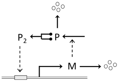
Figure 5.1: Wiring diagram of a bistable molecular switch (Tyson and Novak 2013). The synthesis of protein P is directed by mRNA indicated with M, which is transcribed from a gene controlled by a promoter (gray box on the double-stranded DNA molecule). The promoter is active when it is bound by dimers (or tetramers) of P.

A simple model for this molecular switch is given by the following 2 ODEs:

\[\begin{align} \dfrac{dM}{dt}&=k_{sm} H(P) − k_{dm} M \tag{5.1} \\ \dfrac{dP}{dt}&=k_{sp} M − k_{dp} P \tag{5.2} \end{align}\] where \(M\) and \(P\) represent the concentration of mRNA and protein, respectively, the constants \(k_{sm}\), \(k_{dm}\), \(k_{sp}\) and \(k_{dp}\) represent the rate constants for synthesis and degradation of mRNA and protein, and \(H(P)\) is the probability that the gene encoding the transcription factor is being actively transcribed. Let’s suppose that this probability equals 1 when the transcription factor is bound to the gene’s promoter, and equals \(\epsilon\) when not bound. Then the function \(H(P)\) is commonly taken to be a Hill function:

\[\begin{equation} \tag{5.3} H(P)=\dfrac{\epsilon K_p^n + P^n}{K_p^n + P^n} \end{equation}\] where \(K_p\) is the equilibrium dissociation constant (units of concentration, say nM) of the transcription factor-promoter complex, and \(n\) is the Hill exponent, \(n = 2\) or 4 depending on whether the transcription factor binds to the promoter as a homodimer or homotetramer. The parameter \(\epsilon\) represents the probability that the gene encoding the transcription factor is being actively transcribed at a protein concentration equal to 0 (\(P=0\)).

1. Implement the model as explained in the deBif manual. Use as default starting values of the variables \(M=0.5\) and \(P=0.5\). For the parameters use as default values: \(K_p = 1.0\), \(\epsilon = 0.05\), \(n = 2\), \(k_{sm} = 1.0\), \(k_{dm} = 0.6\), \(k_{sp} = 1.0\) and \(k_{dp} = 0.8\).

2. Use phaseplane() to investigate the dynamics of the model for different initial values of \(M\) and \(P\) between 0.1 and 1.0 for the default parameter values. What stable steady states can you identify?

3. Also study the dynamics with higher and lower values of \(K_p\). What is the effect of changing \(K_p\) on the stable steady states?

4. Use the Steady states tab of phaseplane() to study the change in isoclines when varying the value of \(K_p\) and relate this to the dynamics of \(M\) and \(P\) you observed for these \(K_p\) values.

5. Use the Portrait tab of phaseplane() to study the basin of attraction of the different steady states for different values of \(K_p\). What can you conclude about the basins of attraction?

6. Use bifurcation() to construct the bifurcation graph of the molecular switch model as function of \(K_p\) for otherwise default parameter values. What is the range of \(K_p\) values for which alternate stable states occur?

7. Use bifurcation() to construct the dynamic regime graph of the molecular switch model as function of \(K_p\) and \(\epsilon\). For which values of \(K_p\) and \(\epsilon\) are alternate steady states more prominent?

8. Based on the dynamic regime graph also study the bifurcation graph of the molecular switch model as function of \(K_p\) for a value of \(\epsilon\) for which you expect a qualitatively different graph than for default parameters.

9. Describe how this simple molecular network can operate as an on/off switch.

The above exercises assumed that the transcription factor \(P\) binds to the promoter as a homodimer and hence \(n = 2\). From here on assume that \(P\) binds as a homotetramer to the promotor and therefore adopt \(n=4\).

10. Use the Steady states tab of phaseplane() to study the change in isoclines when varying the value of \(K_p\).

11. Use the Portrait tab of phaseplane() to study the basin of attraction of the different steady states for \(K_p = 1.0\). What can you conclude about the basins of attraction?

12. Use bifurcation() to construct the bifurcation graph of the molecular switch model as function of \(K_p\) for otherwise default parameter values. What is the range of \(K_p\) values for which alternate stable states occur?

13. Use bifurcation() to construct the dynamic regime graph of the molecular switch model as function of \(K_p\) and \(\epsilon\). For which values of \(K_p\) and \(\epsilon\) are alternate steady states more prominent?

14. What can you conclude on the basis of your analysis about the difference in controlling capacity of \(P\) binds as a homodimer or a homotetramer to its promotor?

5.8 Computer practical 6: Cannibalism

The following model describes the dynamics of a cannibalistic population, composed of juveniles \(X\) and adults \(Y\). The adult individuals eat juveniles in addition to alternative food. After scaling the density and time variables the model can be expressed by the following equations:

\[ \begin{split} \dfrac{dX}{dt}&=\alpha\,Y\;-\;X\;-\;X\,Y\\[2ex] \dfrac{dY}{dt}&=X\;-\;\dfrac{\mu}{\rho\:+\:X}\,Y \end{split} \]

in which \(\alpha\) is the (scaled) fecundity of adult individuals; \(\rho\) the (scaled) availability of alternative, non–cannibalistic food for the adults and \(\mu\) represents the constant mortality rate of the adults.

Analyze the model described above, such that you understand as much as possible which type of dynamics the model can exhibit for different parameter values. Use both phaseplane() and bifurcation() to develop this understanding.

Here are some useful guidelines:

1. Use as default parameters: \(\alpha=0.4\), \(\mu=0.05\) and \(\rho=0.05\).

2. Use phaseplane() to construct isocline graphs.

3. To get an initial understanding compute orbits for different starting values of \(X\) and \(Y\). Use \(\rho=0.05\) as parameter value.

4. Construct bifurcation graphs as a function of \(\rho\) for different values of \(\mu\). Sketch these graphs, while indicating which equilibria are stable and which are not.

5. If you encounter any bifurcation points (limit points) construct a graph that shows the location of this bifurcation point as a function of two parameters, for example, as function of \(\mu\) and \(\rho\).

5.9 Computer practical 7: A predator-prey model with density-dependent prey development

Consider a prey population that is subdivided into juveniles and adults. We will denote the densities of juvenile and adult prey by \(J\) and \(A\), respectively. We will assume that adult prey produce offspring at a per capita rate \(\beta\), while juvenile and adult prey die at a per capita rate of \(\mu_j\) and \(\mu_a\), respectively. Both reproduction and mortality are hence density-independent processes. The regulation of the prey population in the absence of any predator is assumed to operate through density-dependent development. The per capita rate of maturation from juvenile to adult is assumed to follow the function:

\[ \dfrac{\phi}{1\,+\,dJ^2} \]

1. Formulate the system of two differential equations describing the dynamics of juvenile and adult prey density \(J\) and \(A\), respectively.

Take as default values for the parameters: \(\beta\) varying between 0.2 and 1.5, \(\phi=1\), \(d=1\), \(\mu_j\) varying between 0 and 0.15 and \(\mu_a=0.2\).

2. Investigate the properties of the model as completely as possible, focusing on the influence of the parameters \(\beta\) and \(\mu_j\).

We will assume that predators, indicated with the variable \(P\), of this prey population only attack adult prey following a linear functional response with an attack rate equal to \(a=1\) (default value). Predators convert the prey biomass they consume into offspring with conversion efficiency \(\epsilon\) equal to 1.0. Predators experience a per capita death rate of \(\delta\) per unit of time.

3. Formulate the system of three differential equations describing the dynamics of juvenile and adult prey density \(J\) and \(A\) their predators \(P\), respectively.

4. Investigate the properties of the model taking \(\delta\) as a bifurcation parameter for different values of \(\beta\) and \(\mu_j\).

5. In total there are 4 different parameter regions to be found, in which the number and type of equilibria differs from the other regions. Try to localize these 4 different areas by computing the boundaries between these regions as a function of \(\beta\) and \(\mu_j\).

Extra: Now assume that in addition to a predator on adults, there is also a predator population, indicated with the variable \(Q\), which exclusively forages on juvenile prey. Again assume a linear functional response with an attack rate symbolized by \(b=1\). Furthermore, assume that the conversion efficiency of this predator on juveniles equals \(m\).

7. Formulate the system of 4 differential equations and investigate its properties.

5.10 Computer practical 8: Lotka-Volterra Predation

The classical equations concerning predator-prey interactions (also: consumer-resource interactions) are:

\[ \begin{split} \dfrac{dR}{dt}&=r\,R\;-\;a\,R\,H\\[2ex] \dfrac{dH}{dt}&=s\,a\,R\,H\;-\;\mu\,H \end{split} \]

And are attributed to Lotka (1932) and Volterra (1926).

Here \(H\) stands for consumers, and \(R\) for resources. \(r\) is the rate of resource replenishment. \(H\) attacks \(R\) with a type I functional response (non-saturating: i.e. constant): \(a\). The conversion rate of sequestered \(R\) biomass to new \(H\) individuals is \(s\), and \(\mu\) is the consumer death rate.

1. What are the possible equilibria? Examine isoclines.

2. Implement the model in R for analysis with phaseplane() and bifurcation() with parameters \(r=0.5\), \(a=0.2\), \(s=0.5\) and \(\mu=0.1\). Examine the stability of the equilibrium to disturbances: is this equilibrium stable? Unstable? Hint: (look at eigenvalues).

3. Examine prey growth in the absence of predators. What do you notice? Is this realistic? Why?

We now assume that resources grow according to the logistic growth model, equilibrating at a carrying capacity \(K\) in the absence of consumption by consumers.

4. What are the equilibria now? What can you say about the feasibility of equilibria? Draw isoclines. How has the stability of the equilibria changed?

5. Implement the model with parameters as above and \(K=10\). How does the model behave differently from the previous one?

6. Examine equilibria as a function of \(K\). Pay special attention to the point `BP'' inbifurcation()`: it marks the intersection of two equilibria, and a subsequent change in stability.

7. Examine the approach to the internal (two-species) equilibrium. What do you notice at small \(K\) (=1.1) and at very large \(K\)?

8. What do you notice about the isoclines at extremely large values of \(K\)? Why does this happen? Link the behavior of the two models.

5.11 Computer practical 9: Neuron activity patterns

Neurons can display a variety of different activity patterns. One prominent activity pattern is tonic spiking, which can be interpreted as a regular train of action potentials. An example of this tonic spiking is shown in the left panel of the figure below. Another example is so-called tonic bursting or chattering, as shown in the right panel below.

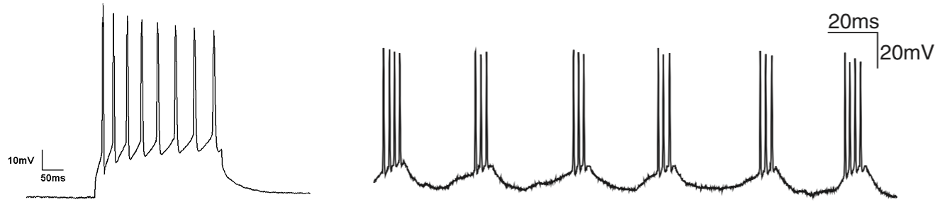
Figure 5.2: Left: Example of tonic spiking. Right: A chattering neuron recorded in vivo from the cat visual cortex shows rhythmic bursting in the gamma frequency range (from Wang 2010).

This computer lab aims at investigating how these different patterns come about and what the dynamic elements are that play a role in generating these patterns.

In a series of classic papers Alan Hodgkin and Andrew Huxley were the first to develop a quantitative model of the propagation of an electrical signal along a squid giant axon (deemed “giant” because of the size of the axon, not the size of the squid). Their model was originally used to explain the action potential in the long giant axon of a squid nerve cell, but the ideas have since been extended and applied to a wide variety of excitable cells. In this computer lab we will focus on a simplified version of the Hodgkin-Huxley model for neuron activity, originally proposed by Hindmarsh and Rose (1984). This Hindmarsh–Rose model (or HR model) of neuronal activity is aimed to study the spiking-bursting behavior of the membrane potential observed in experiments made with a single neuron, as illustrated in the figure above. The model was originally proposed as a system of two ODEs, of which the right-hand side captured in a phenomenological manner results from voltage-clamp experiments with individual neurons (Hindmarsh and Rose 1982). In a later version it was extended to a systems of 3 ODEs, which cn be written in the following form (see Shilnikov and Kolomiets 2008):

The full HR model is given by the following set of three ordinary differential equations: \[\begin{align*} \dfrac{dx}{dt}&= y - a x^3 + b x^2 + I - z\\[2ex] \dfrac{dy}{dt}&= c - d x^2 - y\\[2ex] \dfrac{dz}{dt}&= \epsilon \left(s (x - x_0) - z \right) \end{align*}\] Variable \(x\) represents the voltage across the cell’s membrane, while the ‘gating’ \(y\) and \(z\) variables describe activations or inactivations of some of the currents across the cell membrane. Moreover, the one due to \(z\) is a slow current whose rate of change is of order of the small parameter \(0 < \epsilon \ll 1\). Default parameter values proposed by Hindmarsh and Rose (1984) are: \(a = 1\), \(b = 3\), \(c = 1\), \(d = 5\), \(s = 5\) and \(x_0 = -1.6\). For computational reasons the parameters \(a\), \(c\), \(d\), \(s\) and \(x_0\) will be replaced by their default values as constants in the code of the model implementation. With these default parameters the model is given by the equations: \[\begin{align} \dfrac{dx}{dt}&= y - x^3 + b x^2 + I - z \tag{5.4}\\[2ex] \dfrac{dy}{dt}&= 1 - 5 x^2 - y\tag{5.5}\\[2ex] \dfrac{dz}{dt}&= \epsilon \left(5 (x + 1.6) - z \right) \tag{5.6} \end{align}\]

Of the three remaining free parameters \(I\) represents the external input current, which is in the order of 1 to 3, \(b\) is a design parameter with a default value \(b = 3\) but possibly ranging between 1 and 6 and \(\epsilon\) is the time constant of the slow recovery current, which is in the order of 0.005. The input current \(I\) is probably the most important model parameter since it is linked to experiments (current injection) and in vivo function (synaptic current). It is the only parameter that can vary on a short timescale in experiments and is therefore an obvious, almost imperative, choice as a bifurcation parameter.

1. Implement the model as explained in the deBif manual. To simplify numerical computations introduce only \(I\), \(b\) and \(\epsilon\) as parameters with default values \(I = 1\), \(b = 3\) and \(\epsilon = 0.005\). Base your model implementation therefore on equations (5.4)-(5.6)

2. Analyze the dynamics of the model by constructing time series for \(b=2\) and \(I\) ranging from 1 to 3. Identify the different elements in the dynamic patterns that you observe and explain how they come about.
   Tip: To gain understanding of the dynamics it is useful to only plot the \(x\) and \(z\)-component of the model in your graph with the \(x\)-component on the left \(y\)-axis of the graph and the \(z\)-component on the right \(y\)-axis of the graph.
   Another tip: To gain even more understanding of the dynamics study the dynamics of \(x\), \(y\) and \(z\) in their 3-dimensional phase space using the 3 dimensional plotting option available in bifurcation().

3. Repeat the previous analysis for \(b=3\). Using \(b=3\) also observe what happens if \(\epsilon = 0.001\) is used instead of \(\epsilon = 0.005\). What specific difference do you observe between the dynamics at \(b=2\) and \(b=3\)?

To gain a better understanding about the difference in dynamics of the HR model for \(b=2\) and \(b=3\) we will from here on analyse a simplified version of the HR model in terms of only 2 ODEs. In this simplified HR model the variable \(z\) is now introduced as a parameter and the differential equation for \(dz/dt\) is dropped from the model. The simplified HR model is hence given by the equations: \[\begin{align} \dfrac{dx}{dt}&= y - x^3 + b x^2 + I - z \tag{5.7}\\[2ex] \dfrac{dy}{dt}&= 1 - 5 x^2 - y\tag{5.8}\\[2ex] \end{align}\] with default values \(I = 3\), \(b = 3\) and \(z = 3\).

4. Implement the equations (5.7)-(5.8) of the simplified HR model as explained in the deBif manual. Introduce only \(I\), \(b\) and \(z\) as parameters with default values \(I = 3\), \(b = 3\) and \(z = 3\).

5. Construct the bifurcation graph of the simplified HR model for \(b=3\) as a function of \(z\) for \(I = 1.0\), 2.0 and 3.0. What are the most important dynamical aspects of these graphs? How do the different dynamical regimes that you can identify relate to biological phenomena like the firing patterns shown in the graph above?
   Tip: Use the numerical options tab at the right-hand sidebar to increase the target step size to 0.05, the minimum step size in the bifurcation to 0.01 and the maximum number of points along the curve to at least 2000.

6. Construct the dynamic regime graph of the simplified HR model as a function of \(z\) and \(b\) for the same values of \(I\) used in the previous step. Discuss the effect of changes in \(I\) and changes in \(b\). Can you explain on the basis of the equations of the simplified HR model the effect of changes in \(I\)?

7. Construct the bifurcation graph of the simplified HR model with \(I=3\) as a function of \(z\) for \(b = 1\) and \(b = 2\). What types of dynamical regimes can be identified? Discuss how these types of dynamics relate to the state of the neuron in terms of activity patterns as shown in the the graph above.

8. Now use phaseplane() with \(I = 3\) for \(b = 2\) and \(b = 3\) and different values of \(z\) to study the dynamics in the phase plane of the variables \(x\) and \(y\). Study in particular and describe in detail what happens to the limit cycles in \(x\) and \(y\) with changes in \(z\) when \(b\) equals 2 and when \(b\) equals 3. How does the difference in dynamics that you observed in the original HR model for \(b = 2\) and \(b = 3\) arise and relate to the changes in the limit cycle?
   Tip: Use the Portrait tab of phaseplane()!

5.12 Computer practical 10: The Paradox of Enrichment and its complications

We will examine the effects of an increase of nutrient input into a lake populated by phytoplankton “prey” (\(P\)) and Daphnia “predators” (\(D\)) feeding on phytoplankton.

\[\begin{eqnarray*} \dfrac{dP}{dt}&=&r\,P\,\left(1\:-\:\dfrac{P}{K}\right)\;-\;f(P)\,D\\[2ex] \dfrac{dD}{dt}&=&\epsilon\,f(P)\,D\:-\:\delta\,D \end{eqnarray*}\]

Phytoplankton grows logistically with growth rate \(r\) and carrying capacity \(K\). We assume that phytoplankton are nutrient limited, i.e. that a linear increase in phosphorous and nitrogen levels translates into a linear increase in the equilibrium levels that phytoplankton can attain if growing on their own (\(K\)). \(f(P)\) is a function determining how many phytoplankton are eaten by Daphnia given an encounter, \(\epsilon\) is the conversion efficiency of phytoplankton to Daphnia biomass, and \(\delta\) is the Daphnia death rate.

1. Assume that Daphnia attack phytoplankton according to a satiating, type II functional response. At low prey densities Daphnia are limited by the amount of prey they can find while at high prey densities, Daphnia are limited by the time it takes to handle and digest a prey individual. A function describing this is: \[ f(P)\;=\;\dfrac{a\,P}{1\:+\:a\,T_h\,P} \] with \(a\), the attack rate and \(T_h\) the time it takes a predator to attack and digest a prey individual.
2. Implement the model in R for analysis with phaseplane() and bifurcation(), with parameters \(r=0.2\), \(\epsilon=1\), \(a=0.02\), \(\delta=0.25\), and \(T_h=1\). First examine using phaseplane() the effect of increasing \(K\). What equilibria are possible? Are they stable/unstable? When is coexistence possible? When not? Now examine your findings in bifurcation(). Make several orbits with different initial conditions. What is the effect of increasing carrying capacity?
3. Examine your equilibria as a function of \(K\) in bifurcation().
4. What is a Hopf bifurcation?
5. Point out when a Hopf bifurcation occurs in terms of the configuration of your predator/prey isoclines.
6. What is the “paradox of enrichment”?
7. Why does the paradox of enrichment occur? (In words or in math).
8. Construct the Hopf bifurcation boundary as a function of \(K\) and \(\delta\). This boundary separates the parameter combinations for which limit cycles occur from those for which the equilibrium is stable.
9. Sketch with pen and paper a bifurcation diagram as a function of \(\delta\), based on your \((\delta,K)\)-graph and the bifurcation diagram as a function of \(K\).
10. Use bifurcation() to locate the existence boundary of Daphnia as a function of \(K\) and \(\delta\).
11. A challenge: Use a 3D-plot to visualize the limit cycle as a function of \(K\).

Introducing fish predation

The interactions between Daphnia and phytoplankton lead to destabilization with increasing carrying capacity. The objective in this part will be to examine the robustness of those conclusions to predation pressure by fish (\(C\)) on Daphnia. Fish imposed mortality saturates according to a type III functional response. We assume that fish stocks are constant at \(C\).

\[\begin{eqnarray*} \dfrac{dP}{dt}&=&r\,P\,\left(1\:-\:\dfrac{P}{K}\right)\;-\;f(P)\,D\\[2ex] \dfrac{dD}{dt}&=&\epsilon\,f(P)\,D\:-\:d(D) \end{eqnarray*}\]

in which

\[ f(P)\;=\;\dfrac{a\,P}{1\:+\:a\,T_h\,P} \] and

\[ d(D)\;=\;\delta\,D\:+\:C\,\dfrac{D^2}{1\,+\,A_d\,D^2} \] Use parameters \(r=2\), \(\epsilon=0.5\), \(A_d=44.444\), \(C=6.667\), \(a=9.1463\), \(T_h=0.667\), \(\delta=0.1\).

NB: There is no particular order in the suggestions given under the study questions.

1. Occurrence and stability of equilibria: Start with the qualitative behavior of the model for different levels of productivity (i.e. different values of \(K\), between 0 and 1.0) by studying:

   • Isocline configurations in the phase-plane (use phaseplane()).
   • Time series starting from different initial conditions (use phaseplane() and/or bifurcation()).
   • Bifurcation of equilibria as a function of \(K\).
   • Limit cycles (or the minima and maxima of these) as a function of \(K\).
   • The global behavior of the model. Make sure you have a picture (mentally or on paper) of the isocline configurations in every different region of \(K\).

2. How does the bifurcation graph over \(K\) compare to the system without fish predation on Daphnia as analyzed in the preceding steps of this computer lab? Make an explicit comparison of the bifurcation graphs in the two systems and describe the qualitatively different regions.

3. Effects of predator-induced mortality: Continue with the qualitative behavior of the model for different values of \(C\), by studying:

   • Isocline configurations in the phase-plane (use phaseplane()).
   • Time series starting from different initial conditions (use phaseplane() and/or bifurcation()).
   • Two-parameter bifurcation of all (3 types of) special points found in the bifurcation over \(K\). Deduce from the two-parameter plot a bifurcation graph of the equilibria in the system as a function of \(C\), for different values of \(K\); verify your interpretation with the help of bifurcation().

4. Biological interpretation: What is the effect of a top-predator on the paradox of enrichment?

5.13 Computer practical 11: Chaotic dynamics of Hare and Lynx populations

The following system of ODEs describes the interaction between the hare (\(H\)) that graze the vegetation (\(V\)) and are preyed upon by lynx (\(L\)).

\[ \begin{split} \dfrac{dV}{dt}&=a\,V\,\left(1\:-\:\dfrac{V}{V_{max}}\right)\;-\;a_1\,V\,\dfrac{H}{1\,+\,k_1 V}\\[2ex] \dfrac{dH}{dt}&=a_1\,V\,\dfrac{H}{1\,+\,k_1 V}\;-\;b H - a_2 H L\\[2ex] \dfrac{dL}{dt}&=a_2 H L\;-\;q\,\left(L\:-\:L_{min}\right) \end{split} \]

Take as values for the parameters \(a = 1\), \(V_{max} =150\), \(a_1 =0.2\), \(k_1 = 0.05\), \(b = 1\), \(a_2 = 1\), \(c = 7\) and \(L_{min} = 0.006\).

1. Try to understand the model formulation, in particular the term for the death rate of the lynx. What biological assumption is made for this process?

2. Implement the model in R for analysis with bifurcation() using the parameters above. Use \(V = 7\), \(H = 6\) and \(L = 0.08\) as initial values. Adjust the time series plot to show \(L\) on the \(y\)-axis. Compute a time series with the maximum integration time set equal to 300. Make sure the axes of your graphical window are scaled appropriately.

3. Now change the plot to show all state variables on the \(y\)-axis. Take the scale of the \(y\)-axis equal to 0 to 20. Compute time series with the maximum integration time equal to 300 for \(c = 7.0\), \(c = 7.5\), \(c = 8.0\), \(c = 9.5\) and \(c = 10.2\). Determine the attractor of the system for every one of these \(c\)-values and note the number of minima and maxima. Make sure to distinguish the dynamics of the attractor from the transient dynamics. Which different types of attractors do you find and what type of bifurcation separates these attractors?

4. Change the plot axes to \(V\) on the \(x\)-axis and \(H\) on the \(y\)-axis. Set the plotting range for the \(x\)-axis to 0 to 15 and for the \(y\)-axis equal to 0 to 20 and study the dynamics in this phaseplane.

5. Now turn to a 3D plot of the dynamics with \(V\) on the abscissa, \(H\) on the ordinate and \(L\) on the third axis. Set the plotting range on the \(x\)-axis equal to 0 to 15, on the \(y\)-axis equal to 0 to 12 and on the \(z\)-axis equal to 0 to 1. Compute a time series for \(c = 10.2\) and select the last point of this time series as new initial point. Delete all the curves that you have computed up to now and integrate another time until a maximum integration time of 300. Change the viewing angle of the 3D plot to study the dynamics in more detail.

6. Return to a two dimensional plot with \(L\) on the \(y\)-axis and the range of the \(y\)-axis equal to 0 to 1. Set \(c = 12\) and compute a time series till a maximum integration time of 300, starting from the initial values \(V = 6.8\), \(H = 6.4\) and \(L = 0.015\). Write down the densities of \(V\), \(H\) and \(L\) for \(t = 300\). Now add a very small amount to the initial density of \(V\) (for instance use \(V = 6.800001\)). Compute a new time series without deleting the previously computed one. From which time point onwards do you start to see differences? And how do the densities at \(t = 300\) differ from the previous time series? Also try other nearby starting points (e.g. \(V = 6.800002\)) and see how small changes in the initial value affect the long term prediction. How predictable is this system and how does this predictability depend on \(t\) and on the parameter \(c\)?

7. Study the same time series started from slightly different initial values in a 3D plot of the dynamics with \(V\) on the abscissa, \(H\) on the ordinate and \(L\) on the third axis with the plotting range on the \(x\)-axis equal to 0 to 15, on the \(y\)-axis equal to 0 to 12 and on the \(z\)-axis equal to 0 to 1. Describe the dynamics, and try to explain what causes the unpredictability in the long term dynamics.