Homogeneous Coordinates

The matrix

\[\begin{split}R_\phi = \matvec{cc}{\cos(\phi)&-\sin(\phi)\\ \sin(\phi)&\cos(\phi)}\end{split}\]

rotates a point \((x\; y)\T\) over an angle \(\phi\). The matrix

\[\begin{split}M_y = \matvec{cc}{-1&0\\0&1}\end{split}\]

mirrors a point \((x\; y)\T\) in the vertical (\(y\)) axis. Mirroring and rotation are linear operators that can be represented with a matrix.

Can we also describe a translation with a matrix? The answer is: no, that is not if you kling to the description of a point in 2 dimensional space with a 2 element vector. A matrix describes a linear transformation and therefore the origin should be mapped onto the origin. For a translation this is evidently not true and thus a \(2\times2\) matrix cannot describe translations in a 2D plane.

Homogeneous coordinates in 2D space

Projective geometry in 2D deals with the geometrical transformation that preserve collinearity of points, i.e. given three points on a line these three points are transformed in such a way that they remain collinear. The line may change but the transformed points are again on a line. A translation is a collinearity preserving transformation but it is not a linear transformation and hence there is no \(2\times2\) matrix representing the translation.

The ‘tric’ is to make a 3 component vector out of 2 component vector. Let \((x\;y)\T\) be a vector then we define a homogeneous vector \((sx\;sy\;s)\T\) where \(s\not=0\). When making a homogeneous vector out of a classical vector we often take \(s=1\) meaning that we simply add an extra element equal 1 to the vector. Let \(\v x\) be a vector in \(\setR^2\) then its homogeneous representation is the vector

\[\begin{split}\hv x = \matvec{c}{\v x\\1}\end{split}\]

Given a homogeneous vector \(\hv x\) we may ask what the corresponding 2D vector \(\v x\) is: simple divide by the last element in \(\hv x\) and take the first two elements:

\[\begin{split}\hv x = \matvec{c}{a\\b\\c} \quad \Rightarrow \quad \v x = \matvec{c}{a/c \\ b/c}\end{split}\]

In case \(c=0\) we end up with a point at infinity.

To indicate that two homogeneous vectors \(\hv x\) and \(\hv y\) correspond with the same 2D vector mathematical equality is too strict a demand. The two homogeneous vectors represent the same 2D vector in case there is a scaling factor \(s\not=0\) such that \(s\hv x = \hv y\). We will denote this with:

\[\hv x \sim \hv y \Longleftrightarrow \exists s\not=0: s\hv x = \hv y\]

Rigid Body Transformation

If we now look again at the translation of a vector \((x; y)\T\) over a vector \((t_1\;t_2)\T\) it is easy to prove that this can be written as the matrix vector product:

\[\begin{split}\matvec{ccc}{1&0&t_1\\0&1&t_2\\0&0&1}\matvec{c}{x\\y\\1}\end{split}\]

and the rotation over an angle \(\phi\) can be written as:

\[\begin{split}\matvec{ccc}{\cos(\phi)&-\sin(\phi)&0\\ \sin(\phi)&\cos(\phi)&0\\0&0&1}\matvec{c}{x\\y\\1}\end{split}\]

Combinations of rotations and translations are called rigid body transformations (for obvious reasons). The generic rigid body transformation can be written as:

\[\begin{split}\matvec{ccc}{\cos(\phi)&-\sin(\phi)&t_x\\ \sin(\phi)&\cos(\phi)&t_y\\0&0&1}\matvec{c}{x\\y\\1}\end{split}\]

The rigid body transformations preserve (relative) angles between vectors and they preserve length of vectors. Because angles are preserved, parallelness of lines is preserved.

Note that for a rigid body transformation the resulting scale factor (the third element in the resulting homogeneous vector) is always 1 due to the fact that the bottom row of the transformation matrix has 2 zeros in the first two positions.

Affine Transformations

An affine transform is of the form:

\[\begin{split}A = \matvec{ccc}{a&b&c\\d&e&f\\0&0&1}\end{split}\]

Note that we donote matrices working on vectors in homogeneous representation with a tilde on top. We already know that \((c\; f)\T\) defines a translation. The (sub)matrix

\[\begin{split}\matvec{cc}{a&b\\d&e}\end{split}\]

need not be a rotation matrix. In fact such an affine transform is known to preserve parallelness of lines but angles are not preserved.

Projective Transforms

The most generic case is defined with:

\[\begin{split}P = \matvec{ccc}{a&b&c\\d&e&f\\g&h&1}\end{split}\]

Note that we may choose to set \(P_{33}=1\) because the homogeneous transformation matrix \(P\) and \(a P\) for any \(a\not=0\) have the same interpretation in terms of two dimensional points. We write \(P\sim aP\) to denote this similarity. [1]

Because \(g\) and \(h\) are not both equal zero the third component of a transformed vector need not be 1 and thus the interpretation in terms of a 2D vector does require the division by the third component.

A projective transform is guaranteed to preserve collinearity of points but nothing else.

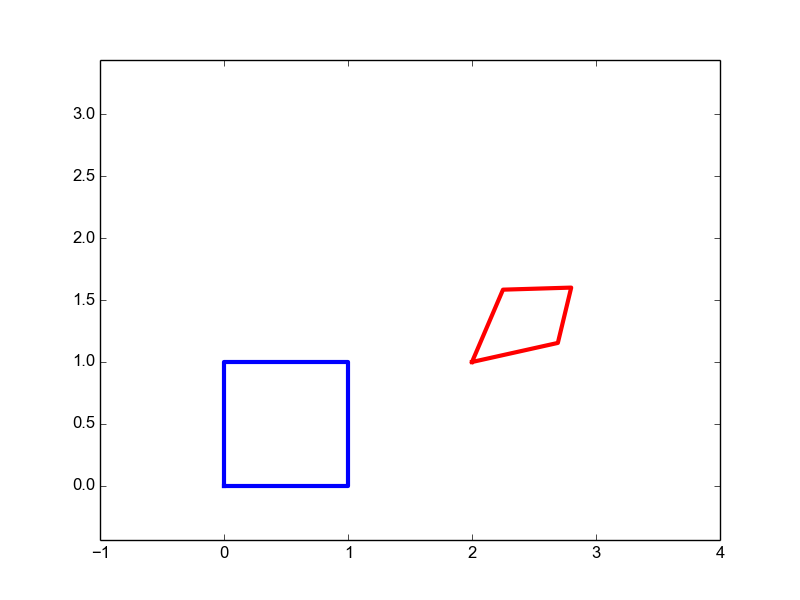
Overview of 2D Transforms

In the table below the basic projective transforms in 2D are given. Please look at the Python code too. Play with the code to sharpen your understanding of the projective transforms encoded in \(3\times3\) homogeneous matrices.

The Degrees of Freedom in the table below indicate the number of parameters that describe the transform. For a translation the dof is 2, for a rotation 1 etc.

Table 1 2D Transforms

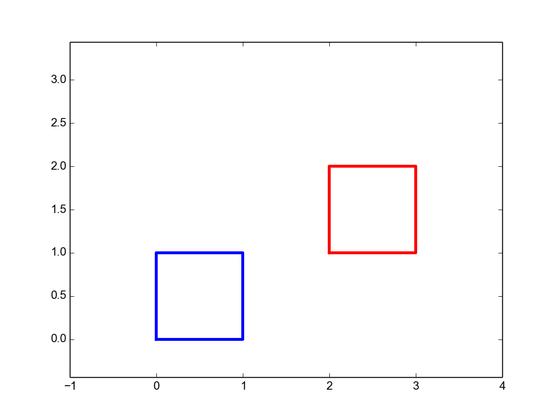
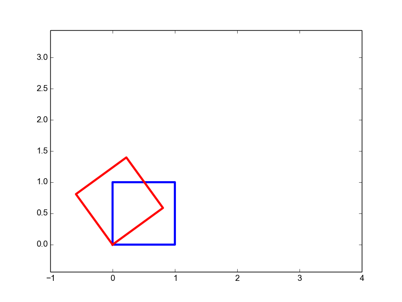
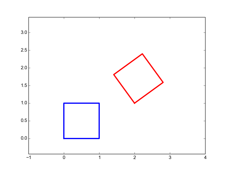
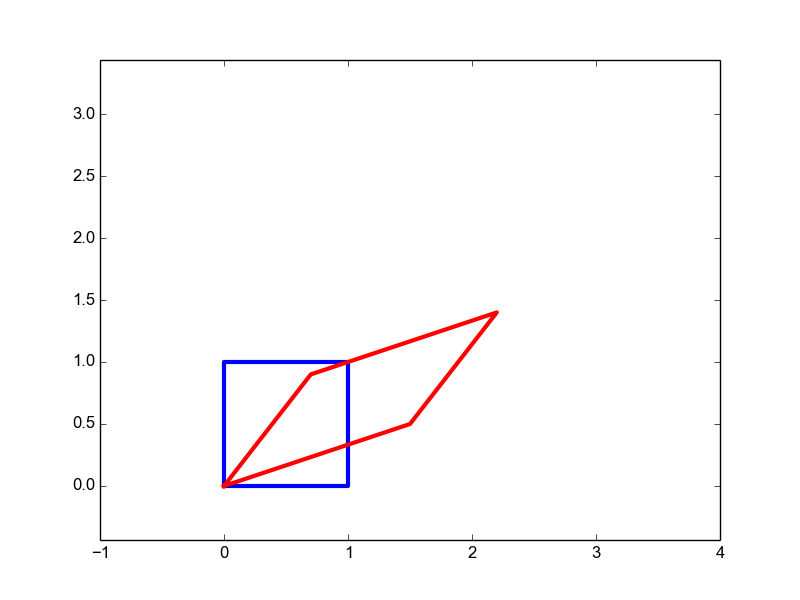
Transform of unit square	Name	Transformation matrix	DoF
	Translation	\(\matvec{ccc}{1&0&t_1\\0&1&t_2\\0&0&1}\)	2
	Rotation	\(\matvec{ccc}{\cos(\phi)&-\sin(\phi)&0\\ \sin(\phi)&\cos(\phi)&0\\0&0&1}\)	1
	Rigid Body	\(\matvec{ccc}{\cos(\phi)&-\sin(\phi)&t_x\\ \sin(\phi)&\cos(\phi)&t_y\\0&0&1}\)	3
	Affine	\(\matvec{ccc}{a&b&c\\d&e&f\\0&0&1}\)	6
	Projective Transform	\(\matvec{ccc}{a&b&c\\d&e&f\\g&h&1}\)	8

Lines in 2D projective space

Using homogeneous coordinates we cannot only describe points in 2D space but also lines in 2D space. The 3 component vector \(\hv l\) represents a line of all points \(\hv x\) (in homogeneous coordinates) such that:

\[\hv l\T \hv x = 0\]

in components we have:

\[\begin{split}\matvec{ccc}{l_1 & l_2 & l_3} \matvec{c}{x\\y\\1} = l_1 x + l_2 y + l_3 = 0\end{split}\]

In case \(l_2\not=0\) we can write:

\[y = - \frac{l_1}{l_2} x - \frac{l_3}{l_2}\]

showing the perhaps more familiar line representation \(y=ax+b\). In geometry the line representation \(\hv l\T\hv x=0\) is prefered as it can represent vertical lines as well.

Given two lines \(\hv l\) and \(\hv m\) the intersection \(\hv x\) of these lines is given by the vectorial cross product:

\[\begin{split}\hv x = \hv l \times \hv m = \determinant{ccc}{ \hv e_1 & \hv e_2 & \hv e_3\\ l_1 & l_2 & l_3\\ m_1 & m_2 & m_3}\end{split}\]

where \(\hv e_1, hv e_2\) and \(\hv e_3\) are the standard basis vectors in 3D space and \(|...|\) denotes the ‘determinant’.

We also have the dual property: two points define a line: let \(\hv x\) and \(\hv y\) be two points then the line passing through these points is given by:

\[\hv l = \hv x \times \hv y\]

An example may illustrate these properties. Consider the points \(\hv a=(3\;2\;1)\T\), \(\hv b=(1\;4\;1)\T\), \(\hv c=(0\;2\;1)\T\) and \(\hv d=(5\;4\;1)\T\). The line \(\hv l\) passes through the points \(\hv a\) and \(\hv b\) so:

\[\begin{split}\hv l &= \hv a \times \hv b\\ &= \matvec{c}{3\\2\\1} \times \matvec{c}{1\\4\\1}\\ &= \determinant{ccc}{ \hv e_1 & \hv e_2 & \hv e_3\\ 3&2&1\\ 1&4&1}\\ &= \hv e_1 (2\times1-1\times4) - \hv e_2 (3\times1-1\times1) + \hv e_3 (3\times4-2\times1)\\ &= -2 \hv e_1 - 2 \hv e_2 + 10 \hv e_3\\ &= \matvec{c}{-2\\-2\\10} = \matvec{c}{1\\1\\-5}\end{split}\]

This is indeed the line \(x+y=5\) as can be easily verified by making a plot. For the line \(\hv m\) through the points \(\hv c\) and \(\hv d\) we have:

\[\begin{split}\hv m &= \hv c \times \hv d = \determinant{ccc}{ \hv e_1 & \hv e_2 & \hv e_3\\ 0&2&1\\ 5&4&1} = -2 \hv e_1 +5 \hv e_2 - 10 \hv e_3 = \matvec{c}{-2\\5\\-10}\end{split}\]

The intersection \(\hv f\) of lines \(\hv l\) and \(\hv m\) is then given by:

\[\begin{split}\hv f = \hv l \times \hv m = \determinant{ccc}{ \hv e_1 & \hv e_2 & \hv e_3\\ 1&1&-5\\ -2&5&-10} = 15 \hv e_1 + 20 \hv e_2 + 7 \hv e_3 = \matvec{c}{15\\20\\7} = \matvec{c}{2.14\\2.86\\1}\end{split}\]

Points at infinity

What also makes the homogeneous representation of points and lines in 2D projective space (represented with homogeneous vectors in 3D space...) special is that we can describe so called points at infinity.

Consider two parallel lines \(\hv l = (a\;b\;c)\T\) and \(\hv m = (a\;b\;d)\T\). Calculating the intersection we get:

\[\begin{split}\hv l \times \hv m = \determinant{ccc}{ \hv e_1 & \hv e_2 & \hv e_3\\ a & b& c\\ a & b& d} = (bd-bc)\v e_1 - (ad-ac)\v e_2 + (ab-ab) \v e_3 = \matvec{c}{b(d-c)\\a(c-d)\\0} = \matvec{c}{b\\-a\\0}\end{split}\]

Note that a normal to the line is given by the 2D vector \((a\;b)\T\) and the 2D point corresponding with homogeneous coordinates \((b\;-a\;0)\T\) is along the direction of the line at infinity.

Coordinate (Frame) Transforms

A point in 2D space can be represented with two numbers \(x\) and \(y\): the coordinates of the point with respect to a basis. Most often when we use the notation \(\v x=(x\;y)\T\) we imply that these coordinates are measured with respect to the standard basis, i.e.:

\[\begin{split}\v x = x\matvec{c}{1\\0} + y\matvec{c}{0\\1}\end{split}\]

Now consider a rotation of the basis vectors over \(\phi\) radians. The rotation matrix \(R\) is given by:

\[\begin{split}R = \matvec{cc}{ \cos\phi & -\sin\phi \\ \sin\phi & \cos\phi}\end{split}\]

The new basis vectors then become

\[\begin{split}R\matvec{c}{1\\0} = \matvec{c}{\cos\phi\\ \sin\phi} \quad\text{and}\quad R\matvec{c}{0\\1} = \matvec{c}{-\sin\phi\\ \cos\phi}\end{split}\]

with respect to this new rotated basis we represent the vector \(\v x\) (that is not changed in space) with coordinates \((x', y')\). We must have:

\[\begin{split}x\matvec{c}{1\\0} + y\matvec{c}{0\\1} &= x'\matvec{c}{\cos\phi\\ \sin\phi} + y'\matvec{c}{-\sin\phi\\ \cos\phi}\\ \matvec{cc}{1&0\\0&1}\matvec{c}{x\\y} &= \matvec{cc}{ \cos\phi & -\sin\phi \\ \sin\phi & \cos\phi} \matvec{c}{x'\\ y'} \\ \matvec{c}{x\\ y} &= R \matvec{c}{x'\\ y'}\end{split}\]

Thus calculating the new coordinates (with respect to the rotated basis) requires the use of the inverse of the basis transform:

\[\begin{split}\matvec{c}{x'\\ y'} &= R\inv \matvec{c}{x\\ y}\end{split}\]

In linear algebra when using a linear transformation, the origin is always mapped onto the origin. Using homogeneous coordinates we can represent translation with a linear operator as well and thus we may shift a coordinate frame in space.

Consider the standard frame and a point with coordinates \((x,y)\). Now consider a frame that is translated with respect to the standard frame such that the origin of the translated frame is at point with coordinates \((a,b)\) (with respect to the standard frame). The frame transform is:

\[\begin{split}F = \matvec{cccc}{ 1 & 0 & a \\ 0 & 1 & b \\ 0 & 0 & 1 }\end{split}\]

We can check this by transforming the origin of the standard frame \((0,0)\), the first basis vector \((1,0)\) and the second basis vector \((0,1)\):

\[\begin{split}F \matvec{c}{0\\0\\1} = \matvec{c}{a\\b\\1} \qquad F \matvec{c}{1\\0\\1} = \matvec{c}{1+a\\b\\1} \qquad F \matvec{c}{0\\1\\1} = \matvec{c}{a\\1+b\\1}\end{split}\]

The coordinate transform is the inverse of the frame transform:

\[\begin{split}F\inv = \matvec{cccc}{ 1 & 0 & -a \\ 0 & 1 & -b \\ 0 & 0 & 1 }\end{split}\]

Consider the frame transform with \((a,b)=(5,3)\). If we want to know what the coordinates are in the translated frame of the point \((6,4)\) (coordinates with respect to the standard frame) we calculate:

\[\begin{split}F\inv \matvec{c}{6\\4\\1} = \matvec{c}{1\\1\\1}\end{split}\]

Now consider the frame transform that is given by:

\[\begin{split}F = \matvec{cc}{ R &\v t\\ \v 0\T & 1}\end{split}\]

where \(R\) is a \(2\times2\) rotation matrix and \(\v t\) is a \(2\times1\) translation vector. The matrix \(F\) thus is of size \(3\times3\). The coordinate transform is the inverse:

\[\begin{split}F\inv = \matvec{cc}{ R\T & -R\T \v t\\ \v 0\T & 1 }\end{split}\]

Estimating Parameters

Affine Transform

An affine transform is described with:

\[\begin{split}\begin{pmatrix}x'\\y'\\1\end{pmatrix} =& \begin{pmatrix}a & b & c\\d & e & f\\0 & 0 & 1\end{pmatrix} \begin{pmatrix}x\\y\\1\end{pmatrix} \\ \hv x' =& A \hv x\end{split}\]

where \((x,y)\) are the coordinates in the input image and \((x',y')\) are the coordinates of the point in the resulting image. Note that the affine transform is invertible

For the affine transform we need to know how three points map to their transformed points (in our case we take 3 corners from a parallelogram in the input image). Let \((x_i,y_i)\) be a point in the input image with corresponding point \((x_i', y_i')\) in the output image.

The relation between between these points and the affine transform matrix can be rewritten in the following form:

\[\begin{split}\begin{pmatrix}x_i'\\ y_i'\end{pmatrix} = \begin{pmatrix}x_i& y_i& 1& 0& 0& 0\\0& 0& 0& x_i& y_i& 1 \end{pmatrix} \begin{pmatrix}a\\b\\c\\d\\e\\f \end{pmatrix}\end{split}\]

The above is just for one point correspondence. For 3 point correspondences we can stack the \(x', y'\) values and also add two rows to the matrix on the right hand side. For three points we have:

\[\begin{split}\begin{pmatrix}x_1'\\ y_1'\\x_2'\\ y_2'\\x_3'\\ y_3'\end{pmatrix} = \begin{pmatrix} x_1& y_1& 1& 0& 0& 0\\0& 0& 0& x_1& y_1& 1\\ x_2& y_2& 1& 0& 0& 0\\0& 0& 0& x_2& y_2& 1\\ x_3& y_3& 1& 0& 0& 0\\0& 0& 0& x_3& y_3& 1 \end{pmatrix} \begin{pmatrix}a\\b\\c\\d\\e\\f \end{pmatrix}\end{split}\]

or:

\[\v q = M \v p\]

The \(6\times6\) matrix \(M\) is invertible (given three non collinear points) and thus:

\[\v p = M\inv \v q\]

In practice it is hard to define the three points with high accuracy, errors will be made. In that case the calculated transform matrix (represented now with the vector \(\v p\)) can be inaccurate. If we are able to find more points correspondences we might be able to obtain a more accurate transform. Say we have \(n\) point correspondences. This leads to a vector \(\v q\) that has \(2n\) elements and a \(M\) matrix that is \(2n\times6\) matrix. Then obviously we cannot simply invert the matrix \(M\) to obtain the transformation matrix characterized with parameter vector \(\v p\).

Instead we solve for a least squares solution for \(\v p\). For a detailed description we refer to Least Squares Estimators. Here we only give the solution:

\[\v p = (M\T M)\inv M\T \v q\]

Note that Numpy has a special function to solve an equation with one line of code:

p = lstsq(M,q)

Projective Transform

The perspective transform is the generic transform characterized with a 3x3 homogeneous matrix:

\[\begin{split}s\begin{pmatrix}x'\\y'\\1\end{pmatrix} =& \begin{pmatrix}a & b & c\\d & e & f\\g & h & i\end{pmatrix} \begin{pmatrix}x\\y\\1\end{pmatrix} \\ \hv x' \sim& P\,\hv x\end{split}\]

Note the scaling factor \(s\) in the above expression which is due to the normalization that is inherent when using homogeneous coordinates (and a transform for which elements \(g\) and \(h\) are not zero). This is also why in the second equation we write \(\sim\) instead of \(=\).

The above can be rewritten as:

\[\begin{split}x' =& \frac{ax+by+c}{gx+hy+i}\\ y' =& \frac{dx+ey+f}{gx+hy+i}\end{split}\]

Make sure you understand that this can be written as:

\[\begin{split}\begin{pmatrix} x & y & 1 & 0 & 0 & 0 & -x'x & -x'y & -x'\\ 0 & 0 & 0 & x & y & 1 & -y'x & -y'y & -y' \end{pmatrix} \begin{pmatrix}a\\b\\c\\d\\e\\f\\g\\h\\i \end{pmatrix} = \begin{pmatrix}0\\0 \end{pmatrix}\end{split}\]

Stacking 4 point correspondences we arrive at:

\[\begin{split}\begin{pmatrix} x_1 & y_1 & 1 & 0 & 0 & 0 & -x_1'x_1 & -x_1'y_1 & -x_1'\\ 0 & 0 & 0 & x_1 & y_1 & 1 & -y_1'x_1 & -y_1'y_1 & -y_1'\\ x_2 & y_2 & 1 & 0 & 0 & 0 & -x_2'x_2 & -x_2'y_2 & -x_2'\\ 0 & 0 & 0 & x_2 & y_2 & 1 & -y_2'x_2 & -y_2'y_2 & -y_2'\\ x_3 & y_3 & 1 & 0 & 0 & 0 & -x_3'x_3 & -x_3'y_3 & -x_3'\\ 0 & 0 & 0 & x_3 & y_3 & 1 & -y_3'x_3 & -y_3'y_3 & -y_3'\\ x_4 & y_4 & 1 & 0 & 0 & 0 & -x_4'x_4 & -x_4'y_4 & -x_4'\\ 0 & 0 & 0 & x_4 & y_4 & 1 & -y_4'x_4 & -y_4'y_4 & -y_4' \end{pmatrix} \begin{pmatrix}a\\b\\c\\d\\e\\f\\g\\h\\i \end{pmatrix} =& \begin{pmatrix}0\\0\\0\\0\\0\\0\\0\\0 \end{pmatrix} \\ \v M \v p =& \v 0\end{split}\]

This is a homogeneous system of equations. It can be shown that in case the points are not colinear there is one non trivial solution for the vector \(\v p\).

In case we have more then 4 point correspondences (and we will when dealing with image mosaics) the matrix \(M\) is of size \(2n\times9\). Then, due to noise in the measurements, there is little chance that there is any null vector. We then set out to find a vector \(\v p\) that minimizes \(\|M \v p\|\) subject to the constraint that \(\|\v p\|=1\) (else the zero vector as trivial solution would suffice). So

\[\min \|M \v p\| \quad\text{s.t.}\quad \|\v p\| = 1\]

Let \(UDV\T\) be the singular value decomposition of \(M\), then:

\[\begin{split}\min \|UDV\T \v p\| \quad\text{s.t.}\quad \|\v p\| = 1\\ \min \|DV\T \v p\| \quad\text{s.t.}\quad \|\v p\| = 1\end{split}\]

due to the fact that \(U\) is orthogonal and therefore preserves the norm. Writing \(\v q = V\T \v p\) we have:

\[\begin{split}\min \|D \v q\| \quad\text{s.t.}\quad \|V \v q\| = 1\\ \min \|D \v q\| \quad\text{s.t.}\quad \|\v q\| = 1\\\end{split}\]

because \(V\) is also orthogonal.

Remember that \(D\) is a ‘diagonal’ matrix with the sorted singular values on the diagonal. Convince yourself that the optimal \(\v q\) then is \(q = (0 0 \cdots 0 1)\T\). And thus \(\v p = V \v q\) which is the last column of \(V\).

Exercises

1. Rigid Body Transformations

   The 2D rotation in homogeneous coordinates is defined with the matrix \(R_\phi\) and the translation is given by the matrix \(T_{\v t}\):

   \[\begin{split}R_\phi = \matvec{ccc}{\cos(\phi)&-\sin(\phi)&0\\ \sin(\phi)&\cos(\phi)&0\\0&0&1}, \qquad T_{\v t} = \matvec{ccc}{1&0&t_1\\0&1&t_y\\0&0&1}\end{split}\]
   1. Calculate the transformation matrix where your first rotate and then translate, i.e. \(T_{\v t} R_\phi\).
   2. Calculate the transformation matrix where you do the reverse: first translate and then rotate.
   3. Is the order in which you do the operations important? Give a numerical example and make a drawing of point \((x\;y)\T\), the result after the first and the result after the second transformation.

2. Invertible transforms

   Let \(T\) be a homogeneous \(3\times3\) matrix. The inverse geometrical transform can be found by inverting the matrix:

   1. Consider a pure translation matrix. Obviously the inverse must be equal to the matrix with negative translation vector. Convince yourself that this indeed true by multiplying \(T_{\v t}\) with \(T_{\v t}^{-1} = T_{=\v t}\).

   2. In case \(T\) is not invertible (i.e. singular), what would you expect to be the shape of the transform of the unit square?

   3. Show that

      \[\begin{split}\matvec{cc}{ R &\v t\\ \v 0\T & 1}\inv = \matvec{cc}{ R\T & -R\T \v t\\ \v 0\T & 1 }\end{split}\]

3. Number of point pairs needed to calculate transformation

   Let \(T\) be a translation. In case we are given a point and its image (i.e. the result of the transform) we can completely determine the transformation. For a translation the DoF equals 2 and thus we need two equations (one for the x-coordinate and one for the y-coordinate) to calculate the translation parameters.

   Calculate the number of corresponding point pairs needed to calculate the parameters of the transformations from the table.

Footnotes

[1]	It is not custom to also denote matrices working on homogeneous vectors with a tilde on top.