Linear Algebra Recap
This is not a chapter where you can learn linear algebra from scratch. It is meant as a way to refresh your linear algebra knowledge. We will only consider the canonical finite dimensional vector space of vectors in \(\setR^n\).
Vectors
A vector \(\v x\) in \(\setR^n\) can be represented with an \(n\)-element vector
each element (also called component or coordinate) \(x_i\) is a real value.
To sharpen your intuition for vectors consider a vector \(\v x\) in two dimensions with elements \(a\) and \(b\). This vector can be interpreted as either:
a point
\(a\) and \(b\) are then the coordinates of a point \((a,b)\) in the plane.
an arrow
\(\v x\) denotes the arrow starting in the origin (the point with coordinates \((0,0)\)) and pointing to the point \((a,b)\).
These interpretations will both be often used in practice.
Linear algebra is called an algebra because it defines way to make calculations with vectors and studies the properties of vectors and calculations with vectors.
The addition of two vectors \(\v x\) and \(\v y\) results in the vector \(\v z\) whose elements are the sum of the corresponding elements of the vectors \(\v x\) and \(\v y\):
The addition of two vectors is easily interpreted as follows (we do a 2D example): take the arrow \(\v x\) and draw it starting at the origin, next draw the arrow \(\v y\) but start at the end point of \(\v x\). These ‘concatenated’ arrows then end at the point \(\v z\).
The scalar multiplication of a vector \(\v x\) with a scalar \(\alpha\) (i.e. a real value) is defined as the elementwise multiplication with \(\alpha\):
Consider again the two dimensional example of the vector \(\v x\) with elements \(a\) and \(b\). The vector \(\alpha \v x\), with \(\alpha>0\) then is a vector in the same direction as \(\v x\) but with a length that is \(\alpha\) times the original lenght.
For \(\alpha>1\) the length is increased, for \(0<\alpha<1\) the length is decreased. But what happens when we take a negative \(\alpha\)? Consider the case:
Indeed the direction is reversed, the vector now points in the opposite direction.
Note that vector subtraction \(\v x - \v y\) simply is \(\v x + (-\v y)\).
The zero-vector \(\v 0\) is the vector of which all elements are zero. Remember from classical algebra that for any scalar \(a\) we have \(a+0=a\). For the zero vector we have that for each vector \(\v x\) it is true that: \(\v x + \v 0=\v x\).
Vector addition is commutative, i.e. \(\v x + \v y = \v y + \v x\).
Vector addition is associative, i.e. \((\v x + \v y) + \v z=\v x + (\v y + \v z)\).
Both these properties together imply that in a summation of vectors the order and sequence of the additions are irrelevant: you may leave out all brackets and change the order of vectors.
Basis Vectors
Consider the 2D vector \(\v x=\matvec{cc}{3&2}\T\) [1]. When we draw it in a standard coordinate frame we mark the point that is 3 standard units from the right of the origin and 2 units above the origin.
Note that the vector \(\v e_1 = \matvec{c}{1&0}\T\) is pointing one unit in the horizontal direction and the vector \(\v e_2=\matvec{c}{0&1}\T\) is pointing one unit in the vertical direction. The vector \(\v x\) may thus be written as:
In general a vector \(\matvec{cc}{a&b}\T\) can be written as \(a\v e_1+b\v e_2\). The vectors \(\v e_1\) and \(\v e_2\) are said to form a basis of \(\setR^2\): any vector in \(\setR^2\) can be written as the linear combination of the basis vectors.
But are the vectors \(\v e_1\) and \(\v e_2\) unique in that sense? Aren’t there other vectors say \(\v b_1\) and \(\v b_2\) with the property that any vector can be written as a linear combination of these vectors? Yes there are! Any two vectors \(\v b_1\) and \(\v b_2\) that do not point in the same (or opposite) direction can be used as a basis.
For instance take \(\v b_1=\matvec{cc}{1&1}\) and \(\v b_2 = \matvec{cc}{-1&1}\) then we have that:
as can be checked by working out the vector expression in the right hand side of the above equality.
Linear Mappings
A linear mapping is a mapping \(\op L\) that takes a vector from \(\setR^n\) and maps it on a vector from \(\setR^m\) such that:
Consider a mapping \(\op L\) that takes vectors from \(\setR^2\) and maps these on vectors from \(\setR^2\) as well. Remember that any vector in \(\setR^2\) can be written as \(\v x = x_1 \v e_1 + x_2 \v e_2\), then:
Note that \(\op L \v e_1\) is the result of applying the mapping on vector \(\v e_1\), by choice this is a vector in \(\setR^2\) as well and therefore there must be two numbers \(L_{11}\) and \(L_{21}\) such that:
Equivalently:
So we get:
Let \(\op L\v x = \matvec{cc}{x'_1&x'_2}\T\) be the coordinates with respect to the elementary basis, then we have:
The four scalars \(L_{ij}\) for \(i,j=1,2\) thus completely define this linear mapping. It is customary to write these scalars in a matrix:
For now a matrix is a symbolic notation, we will turn matrices and vectors into a real algebra in the next subsection when we consider calculations with matrices and vectors. With the matrix \(L\) we can define the matrix-vector product that describes the relation between the original vector \(\v x\) and the resulting vector \(\v x'\):
or equivalently:
Note that we may identify a linear mapping \(\op L\) with its matrix \(L\) (as is often done) but then carefully note that the basis for the input vectors and the basis for the output vectors are implicitly defined.
Matrices
A matrix \(A\) is a rectangular array of numbers. The elements \(A_{ij}\) in the matrix are indexed with the row number \(i\) and the column number \(j\). The size of a matrix is denoted as \(m\times n\) where \(m\) is the number of rows and \(n\) is the number of columns.
Matrix Addition. Two matrices \(A\) and \(B\) can only be added together in case both are of size \(m\times n\). Then we have:
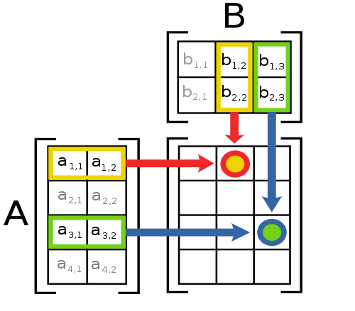
Fig. 1 Figure from Wikipedia.
Matrix Multiplication Two matrices \(A\) and \(B\) can be multiplied to give \(C=AB\) in case \(A\) is of size \(m\times n\) and \(B\) is of size \(n\times p\). The resulting matrix \(C\) is of size \(m\times p\). The matrix multiplication is defined as:
Matrix-Vector Multiplication. We may consider a vector \(\v x\) in \(\setR^n\) as a matrix of size \(n\times 1\). In case \(A\) is a matrix of size \(m\times n\) the matrix-vector multiplication \(A\v x\) results in a vector in \(m\) dimensional space (or a matrix of size \(m\times 1\).
In a previous section we have already seen that any linear mapping from \(n\) dimensional vector space to \(n\) dimensional vector space can be represented with a \(m\times n\) matrix.
Dot Product. Consider two vectors \(\v x\) and \(\v y\) both in \(\setR^n\), then the dot product is defined as the sum of the multiplications of the elements of both vectors:
note that we can also write:
Matrix Transpose. Consider a matrix \(A\) of size \(m\times n\), then the transpose \(A\T\) is the matrix where the rows and columns of \(A\) are interchanged:
note that \(A\T\) has size \(n\times m\). The transpose is the operator that turns a column vector into a row vector (and vice versa).
Symmetric Matrices. In case \(A\T = A\) the matrix \(A\) is called symmetric.
Square Matrices. A matrix is square if \(m=n\).
Diagonal Matrix. A square matrix with only non zero elements on the main diagonal (i.e. the elements \(A_{ii}\)).
Identity Matrix. The diagonal matrix with all diagonal elements equal to one. The diagonal matrix of size \(m\times m\) is denoted as \(I_m\) (the size subscript is omitted in case this is clear from the context).
Interpreted as a linear mapping, the identity matrix corresponds with the identity mapping (i.e. \(I\v x = \v x\) for all \(\v x\)).
Linear Equations, Determinants and Inverse Matrices
The matrix-vector equation \(A\v x= \v b\) where \(A\) is a known matrix of size \(m\times n\), \(\v x\) is the unknown column vector of size \(n\times 1\) and \(\v b\) is a known vector of size \(m\times 1\), defines a set of \(m\) equations in \(n\) unknowns:
A necessary condition for such a set of equations to have a unique solution is that \(m=n\), i.e. is \(A\) is a square matrix.
In case the determinant \(|A|\) is not equal to zero the matrix is called non-singular and an inverse matrix \(A\inv\) exists. For the inverse of a matrix \(A\) (if it exists) we have that \(A A\inv = A\inv A = I\).
A set of linear equations and represented with \(A\v x = \v b\) thus has a solution \(\v x = A\inv \v b\). Please note that solving a set of linear equation by calculating the inverse matrix is not a wise thing to do. Better ways to solve such a system are known and available in most linear algebra packages.
Vector Norm, Inner Products and Orthogonality
Let \(\v x\) be a vector in 2D space with coordinate representation \(\v x = \matvec{cc}{x_1&x_2}\T\) with respect to orthogonal basis vectors of unit length (i.e. an orthonormal basis), then we may use Pythogoras’ theorem to calculate the length of the vector, which is denoted as \(\|\v x\|\) and is called the vector norm:
The inner product \(\langle \v x, \v y \rangle\) of two vector \(\v x\) and \(\v y\) relates the length of the vectors with the angle between the vectors:
In a vector space where the coordinates are relative to an orthonormal basis we have that
In case the angle between the two vectors is \(90\) degrees (or \(\half\pi\) radians), i.e. the vectors are orthogonal, we have that \(\v x\T\v y=0\).
An \(n\times n\) matrix \(A\) whose columns form an orthonormal basis is called an orthogonal matrix. Interpreted as linear mappings an orthogonal matrix preserves the length (norm) of vectors: \(\|A\v x\|=\|\v x\|\). The inverse of an orthogonal matrix equals the transpose: \(A\inv = A\T\).
Eigenvectors and Eigenvalues
Consider a linear mapping from \(\setR^n\) onto itself. Such a mapping can be represented with a square \(n\times n\) matrix \(A\). In case for a specific vector \(\v x\) we have that:
we say that \(\v x\) is an eigenvector of \(A\) with corresponding eigenvalue \(\lambda\).
Let \(A\) be a symmetric \(n\times n\) matrix then it can be shown that there are \(n\) eigenvectors that form an orthonormal basis of \(A\). Let \(\v u_i\) for \(i=1,\ldots,n\) be the \(n\) eigenvectors with corresponding eigenvalues \(\lambda_i\) then we can write:
where \(U = \matvec{c}{\v u_1,\ldots,\v u_n}\) is the matrix whose columns are the \(n\) eigenvectors and \(D\) is a diagonal matrix whose entries are the corresponding eigenvalues. The above equation is called the eigenvalue decomposition.
Singular Value Decomposition
Given any matrix \(A\), the singular value decomposition (SVD) writes the matrix as a product of a orthogonal matrix \(U\), a ‘diagonal’ matrix \(D\) and a second orthogonal matrix \(V\):
Evidently the matrix \(D\) cannot be truly diagonal in general as \(A\) is not necessarily a square matrix. It is nevertheless called diagonal because only the elements \(D_{ii}\) can be different from zero.
| [1] | The \(\v x\T\) denotes the transpose of a vector. For now you can read it as a way to make a column vector out of a row vector. |