Multivariate Functions
In programming we are accustomed to the fact that a function may take more then one argument to produce a result. For mathematical functions we also have functions with more then one argument: multivariate functions. As a simple example consider
Plotting a multivariate function
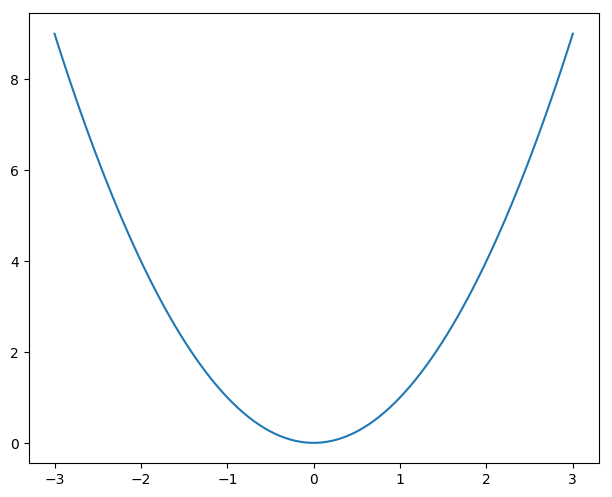
For a univariate function (one argument) plotting the graph of the function is easy. These are the function plots that you are all familiar with.
In [1]: from pylab import *;

In [2]: x = linspace(-3,3,100);

In [3]: clf(); plot(x, x**2);
Multivariate functions in two arguments (we will call them 2D functions) are possible (given our capabilities of interpreting 2D drawings of 3D objects).
In [4]: from mpl_toolkits.mplot3d import Axes3D;

In [5]: x,y = meshgrid(linspace(-3, 3, 50), linspace(-3, 3, 50));

In [6]: z = x**2 + y;

In [7]: fig = figure(); ax = Axes3D(fig);

In [8]: ax.plot_surface(x, y, z, linewidth=0, cmap=cm.copper, rstride=1, cstride=1, shade=True);
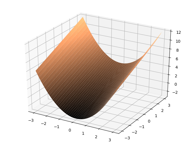
The shape of this wireframe surface is easy to understand from the function recipe. For a \(y=0\) we have \(f(x,0)=x^2\) and as a function of \(x\) that is the parabola. For any value \(y=a\) we have a parabola in \(x\): \(f(x,a)=x^2+a\). For any value \(x=a\) we have straight line in \(y\): \(f(a,y)=a^2+y\).
Math doesn’t end with 2D functions. In fact in many branches of computer science (statistical learning techniques for example) functions with hundreds of arguments are quite common. But our methods of visualizing multivariate functions do end with 2D functions. Beyond that function (data) visualization becomes interpretation too, we have to select how to render the information in a 3D space that can be visualized. We refer to lectures on scientific visualization.
Differentiating a multivariate function
Remember the derivative of a univariate function:
So the derivative measures something like the rate of change. It gives the change in value when we change the argument a little bit. Derivatives are therefore the mathematical way of describing change. For a univariate function the derivative at \(x=a\) is the slope of the tangent line to the function in \((a,f(a))\).
The derivative of a function \(f\) is also a function. Taking the derivative thus transforms a function into a new function. The derivative function is often denoted as \(f'\).
We can take the derivative of the derivative. Then we calculate the change in the slope as we move a little along the horizontal axis. The second derivative is denoted as \(f''=\frac{d^2f}{dx^2}\). In the same way we can calculate the derivative up to any order (3th, 4th etc).
Differentiating a multivariate function is somewhat more complex. The idea is the same: what happens to the function value when i change the input just a little? But what do i mean now with changing the input? Should all the arguments be changed, or just one? Well actually it is your choice, there is a need for both these options in practice.
The simplest one is to change only one of the arguments and see what happens to the function value. Consider the function \(f\) in two arguments, say \(x\) and \(y\). Let us change \(x\) to \(x+h\), while keeping \(y\) fixed! We could then calculate what is known as the partial derivative of \(f\) with respect to its first argument which is called \(x\).
Observe that instead of \(df/dx\) we write \(\partial f/\partial x\) to distinguish between the derivative of a univariate function and the derivative with respect to just one argument (the one that by convention is called \(x\)) of a multivariate function. Be sure to understand that the partial derivative of a multivariate function results in a multivariate function in the same number of arguments.
The partial derivative in the \(y\) argument is:
At high school you have learned how to calculate the derivatives of functions. Better said you were given the derivatives of some basic functions (like \(x^n\), \(\cos(x)\), \(\log(x)\) and others) and the rules to calculate the derivatives of compound functions (like the chain rule and the product rule). Can we use this knowledge for partial differentiation as well? Yes we can. Remember when we are (partially) differentiating \(f\) with respect to \(x\) we keep \(y\) fixed and thus while differentiating anything in the formula with a \(y\) in it, it is treated as a constant.
For instance consider \(f(x,y)=x^2+y\). Differentiating with respect to \(x\) leads to \(2x\). The rules to follow here are:
- the derivative of a sum is the sum of the derivatives, so we may take the derivative of \(x^2\) plus the derivative of \(y\).
- the derivative of \(x^2\) with respect to \(x\) is equal to \(2x\)
- the derivative of \(y\) with respect to \(x\) is \(0\).
The partial derivative with respect to \(y\) is a constant function equal to \(1\) everywhere (note that the term \(x^2\) now is taken to be fixed, i.e. constant with zero derivative).
Also for partial derivatives we may repeat the differentiation. So the second order derivative in the \(x\) argument is denoted as \(\partial^2 f / \partial x^2\). But now we can do something else as well: first take the derivative in \(x\) direction followed by taking the derivative in \(y\) direction. Or the other way around: first \(y\) then \(x\). It can be shown that for most functions the order in which the derivatives are taken does not matter. We have:
The partial derivatives play an important role in the analysis of local structure in images. To make notation a bit simpler there we will use the subscript notation for partial derivatives. Let \(f\) be a 2D function with arguments we name \(x\) and \(y\). The partial derivative with respect to \(x\) is denoted as \(f_x\), and the second partial derivative both with respect to \(x\) as \(f_{xx}\). The mixed second order derivative if \(f_{xy}\).
We will also sometimes use the notation \(\partial_x\) to denote \(\frac{\partial}{\partial x}\).
The order of differentiation of a multivariate function is the total number of times we do a differentiation not matter in which argument. So \(f_x\) and \(f_y\) are first order derivatives, whereas \(f_{xx}\), \(f_{xy}\) and \(f_{yy}\) are second order derivatives. Note that \(f_{xxy}\) is a third order derivative.
Exercises:
Calculate all partial derivatives up to order 2 of the functions:
\[\begin{split}\begin{gather} f(x,y) = \exp\left( - a(x^2+y^2) \right)\\ g(x,y) = \cos(a x + b y) \end{gather}\end{split}\]i.e. calculate \(f_x\), \(f_y\), \(f_{xx}\), \(f_{xy}\) and \(f_{yy}\) and the same derivatives but then for the function \(g\).
Given:
\[g(x,y,s) = \frac{1}{2\pi s^2}\exp\left( -\frac{x^2+y^2}{2s^2} \right)\]calculate \(g_s = \partial_s g = \frac{\partial g}{\partial s}\).
Symbolic Math Computations
Computer scientists are (in most cases) no mathematicians. So doing a lot of tedious, error prone math (be it calculus, linear algebra or any other branch) is not our joy in life. Fortunately there are symbolic math programs to solve most of our day to day needs.
There are many great programs for symbolic math. Mathematica is perhaps the best known. Mathematicians themselves tend to use Maple more in my perception. Other symbolic math programs do exist.
Here we will use SymPy that is an extension for Python to deal with some simple symbolic math.
In [9]: from sympy import *
In [10]: x = Symbol("x"); y = Symbol("y"); a = Symbol("a");
In [11]: f = x**2+y;
In [12]: diff(f, x)
Out[12]: 2*x
In [13]: diff(f, y)
�������������Out[13]: 1
In [14]: diff(f, x, 2)
������������������������Out[14]: 2
In [15]: f = exp(-a*(x**2+y**2));
In [16]: diff(f,x,1)
Out[16]: -2*a*x*exp(-a*(x**2 + y**2))
In [17]: diff(f,y,1)
��������������������������������������Out[17]: -2*a*y*exp(-a*(x**2 + y**2))
In [18]: simplify(diff(f,x,2))
����������������������������������������������������������������������������Out[18]: 2*a*(2*a*x**2 - 1)*exp(-a*(x**2 + y**2))
In [19]: simplify(diff(f,x,1,y,1))
������������������������������������������������������������������������������������������������������������������������������Out[19]: 4*a**2*x*y*exp(-a*(x**2 + y**2))
In [20]: simplify(diff(f,y,2))
������������������������������������������������������������������������������������������������������������������������������������������������������������������������Out[20]: 2*a*(2*a*y**2 - 1)*exp(-a*(x**2 + y**2))