2.1. Colorimetry
\(\newcommand{\la}{\lambda}\)
A ray of light that hits the photosensitive cells in the retina is physically characterized by its spectral distribution \(t\) as a function of the wavelength \(\la\), i.e. \(t(\la)d\la\) is the energy in the beam due to the light with wavelengths in the interval from \(\la\) to \(\la+d\la\). In colorimetry, the science of color measurements, we study beam colors, i.e. the colors associated with beams of light. This in contrast with object colors, the colors associated with objects that reflect the light from an illumination source. When a red apple is illuminated with a beam of white light, the apple only reflects the red components of the light, this makes the apple appear to be red. Illuminating the apple with light containing no red light makes the apple appear black; there is no red light to reflect. Choosing different colored beams to illuminate the ‘red’ apple its perceived color can change dramatically. Nevertheless we talk about the ‘red’ apple with good reason. The material properties of the apple make it appear red to the eye when illuminated by white light.
2.1.1. The physics of color
What we call light is electromagnetic radiation with wavelengths in a small part of the entire range; the photo receptors in the retina are sensible to the electromagnetic waves with wavelength in the interval from about 400 to 700 nm only.

Fig. 2.1 The electromagnetic spectrum. Note that the visible spectrum comprises only a small part of the total spectrum of electromagnetical waves.
It is the spectral distribution function or spectrum of a ray of light that completely characterizes a beam (and thus its color) within the colorimetric context. Because the spectrum \(t\) as function of the wavelength \(\la\) is a function over the real numbers, the ‘space’ of all spectra is infinite dimensional. [1]
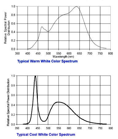
Fig. 2.2 Two examples of spectra. Both colors appear to the eye as shade of white.
In this chapter we follow the standard colorimetric practice to represent a spectrum (and any other function of \(\la\)) with its sampled version. Let \(f\) be a function of \(\la\) then we represent \(f\) with its sampled version \(F\), where \(F(k)=f(\la_k)\). Most often the sampling points are taken 5 nm (or 10 nm) apart where \(\la_k\) runs from about 400nm to 700nm.
For color spectra it is very advantageous to represent the collection of samples \(F(k)\) with a vector \(\v f\) with elements \(f_k=F(k)\). We assume that spectral ‘vectors’ are in a \(N\)-dimensional space. With this representation of spectra (and colors to be introduced shortly) as vectors we can utilize the mathematical tools from linear algebra [2].
2.1.2. The perception of color
Within the retina of the human eye two basic classes of photo receptors can be found: the rods and cones. The rods are used in low light level conditions. The rods are not capable of distinguishing different colors; only light dark differences are detectable.
The second class of photo receptors are the cones. These are concentrated in the center of the visual field (the fovea). There are three types of cones. These contain photosensitive pigments with different spectral absorptances. Let \(t\) be the spectral distribution of the beam incident on the retina, the response of the i-th type of cone with sensitivity \(s_i\) is given as:
In the figure below the three sensitivity functions are shown. They are also known as the \(S\), \(M\) and \(L\) sensitivity curves as they roughly correspond with the short, medium and long wavelength electromagnetic waves.
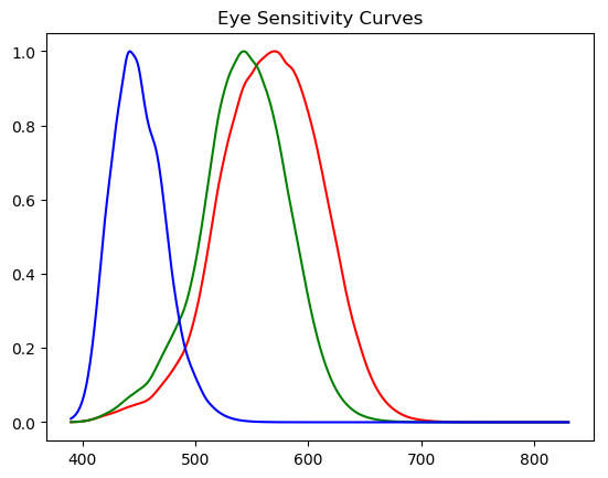
Although in the figure the curves are colored blue, green and red (from left to right) corresponding with their placement in the range of spectral colors, it is more accurate to name them the small, medium and large wavelength sensitivity curves.
Also note that each of the curves is scaled to have a maximum value of 1. In reality the small wavelength curve is less sensitive (a lower maximal value) then the two other curves. The human eye is least sensitive to blue light.
Within the vector representation of spectra and sensitivity functions an approximation of the above integral expression becomes:
i.e. the inner product of the sensitivity and the spectrum [3]. Combining the three responses \(c_i\) for \(i=1,2,3\) in one tristimulus response vector \(\v c\) we get:
where \(S\) is the sensitivity matrix whose columns are the 3 sensitivity vectors \(S = ( \v s_S \, \v s_M \, \v s_L )\). The matrix \(S\T\) is the representation of a mapping from the \(N\)-dimensional spectral space onto the 3D tristimulus vector space.
The tristimulus vector \(\v c\) is the input to the brain for any beam of uniform colored light that hits the retina. Thus two beams with spectra \(\v t_1\) and \(\v t_2\) appear to be equally colored in case
Carefully note that this doesn’t mean that the two spectra are equal. The mapping \(S\T\) from a high (\(N\)) dimensional space onto a 3 dimensional space does not have an inverse and therefore \(S\T \v t_1 = S\T \v t_2\) does not necessarily imply that \(\v t_1=\v t_2\). Spectra that give rise to the same color tristimulus values are called metameric spectra. Metamerism is both a cause of a lot of difficulties in color science but also of great practical importance.
2.1.3. Spectral versus Color Space
All possible spectra form what we call spectral space \(\set S\). Essentially this is a infinite dimensional vector space (the vectors are functions). Sampling the spectra leads to a finite dimensional spectral space. The dimension of space of sampled spectra equals the number of samples of the spectrum.
Not every (mathematical) point in spectral space is a valid spectrum: spectra are always positive functions and thus only the positive ‘hyper octant’ of the space represents the physical spectra.
A spectrum vector \(\v t\) is mapped onto a 3 dimensional vector \(\v c = S\T \v t\) in color space. As the \(S\) matrix also contains only positive elements \(\v c\) also lies in the first octant of 3D color space. But even that positive octant is not completely filled, i.e. not every positive vector \(\v c\) represents a color (i.e. projected positive spectrum).
The figure below shows the cone of all “real” colors in color space. This cone can be easily constructed as set of all convex combinations of all colors \(S\T \v e_i\) where \(\v e_i\) are the monochromatic spectra (i.e. a vector from the standard basis of spectral space).
2.1.4. Chromaticity Coordinates
It is an empirical fact that color response is linear. I.e. when we mix two beams of light with spectra \(\v t_1\) and \(\v t_2\) then the mixed beam has a spectrum \(\v t_1+\v t_2\) and the color response is indeed \(\v c_1+\v c_2\). This is also in accordance with a linear model \(\v c=S\T \v t\) for we have \(S\T(\v t_1+\v t_2)=S\T\v t_1 + S\T\v t_2 = \v c_1 + \v c_1\).
A second empirical fact is that the color of a beam does not perceptually change when its intensity is changed. Thus a beam with spectrum \(\v t\) and a beam with spectrum \(a \v t\) only differ in perceived brightness, not in color.
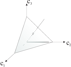
Fig. 2.3 Chromaticity plane
Consider a half line emanating from the origin in the tristimulus space. All points on this line can be written as \(a \v c_0\) where \(\v c_0\) is a point on this line. All the points on the line have the same color, only the perceived brightness is different. Therefore the color may be characterized uniquely with the intersection of the half line with a plane. In the figure above we have sketched the plane \(c_1+c_2+c_3 =1\) as an example of such a chromaticity plane. Please note that the chromaticity plane is not necessarily a plane of equal intensity beams!
We don’t need three coordinates to identify a color in the chromaticity plane. Just two coordinates, say \(c_1\) and \(c_2\) are enough (why?). The plot of colors in a two dimensional view of the chromaticity plane is called a chromaticity diagram.
There is nothing special or magical about chromaticity diagrams. Instead of defining a chromaticity plane we could equally well take any parameterizable surface such that all half lines intersect the surface only once. The disadvantage of such a choice is that additive color mixtures are not easily represented as linear mixtures in the chromaticity plane anymore.
2.1.5. Color matching experiment
Consider again the color match of the two beams \(\v t_1\) and \(\v t_2\), i.e.\(S\T \v t_1 = S' \v t_2\). Let \(A\) be any non-singular \(3\times3\) matrix then \(S\T \v t_1 = S\T \v t_2 \Leftrightarrow A\T S\T \v t_1 = A\T S\T \v t_2\). This shows that for color matching experiments any linear combination of the sensitivity curves of the human eye will lead to the same color matches. Any matrix \(C=S A\) is called a color matching matrix.
In fact color matching matrices were the basis of colorimetry long before the human sensitivity matrix could be measured directly and accurately. Understanding color matching experiments is therefore crucial in understanding the international standards in color representation.
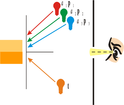
Fig. 2.4 Color Matching. In a color matching experiment the observer sees a (circular) field of two halves. In one half the test light (spectrum \(\v t\)) is shown. In the other half a mixture of three primaries is shown. The observer is asked to set the attenuation of the three primary beams to obtain a perceptual match of the two colors.
In a color matching experiment an observer looks at a circular field composed of two halves. From one half of the field the arbitrary beam with spectrum \(\v t\) is visible and from the other half the mixture with spectrum \(\v u\) of three fixed lights (the primaries) is visible.
Let the spectra from the three primaries at full intensity be \(\v p_1\), \(\v p_2\) and \(\v p_3\). The three primaries should be colorimetric independent, i.e. the associated tristimulus vectors \(S\T \v p_1\), \(S\T \v p_2\) and \(S\T \v p_3\) should be linearly independent.
The observer can control the attenuation factor \(a_i\) of each of the primaries. This results in an observed spectrum \(\v u=a_1 \v p_1 + a_2 \v p_2 + a_3 \v p_3\). The observer is asked to control the attenuation factors such that the color in both halves of the circular field appear to be equal. Such a color match requires that:
Collecting the three primaries in one matrix \(P = ( \v p_1\, \v p_2\, \v p_3 )\) and writing the attenuation factors in a vector \(\v a= (a_1\, a_2\, a_3)'\), the color match equation can be written as:
Because \(S\T P\) is invertible we get:
showing that for any spectrum \(\v t\) we can find the attenuation factors \(\v a\) to construct a color match using any three (colorimetric independent) primaries.
Some test lights to be matched lead to negative attenuation factors according to Eq. (1). Negative attenuation factors are of course a physical impossibility. The color matching experiment is not lost though. If we shift the primary beam with the negative factor to the side of the unknown light source we have a positive factor again. The observed colors will change because we add a second source to the test beam. A color matching experiment is concerned with color equivalence and not with color appearance.
Note that the matrix \(C\T = (S\T P)^{-1} S\T\) needed to calculate \(\v a\) given the spectrum \(\v t\) is of the form \(A S\T\) where \(A\) is a \(3\times3\) non-singular matrix. It has already been argued that such a matrix leads to equivalent color matches as the human sensitivity matrix.
The solution for the attenuation factors \(\v a\) to match a color beam \(\v t\) in the form given in (1) is dependent on the human sensitivity matrix \(S\), for we have \(\v a=C\T \v t = (S\T P)^{-1} S\T \v t\). The matrix \(C\T = (S\T P)^{-1} S\T\), however, can be measured directly without knowing \(S\) explicitly. The human observer (‘who has the matrix \(S\) in his brain’) is needed to judge color equivalence.
Let \(\v t=\v \Delta_i\) be the spectrum of a monochromatic beam of wavelength \(\la_i\). The monochromatic beam \(\v \Delta_i\) has a unit vector representation:
where the \(1\) element is at index \(i\) in the vector.
Then \(\v a=C\T \v t\) is the \(i\)-th row of the color matching matrix \(C\). Thus by repeating the color matching experiment for all monochromatic beams the entire color matching matrix \(C\) can be determined experimentally. The color matching matrix is dependent on the chosen primary beams.
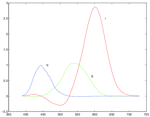
Fig. 2.5 Color matching functions. In this experiment monochromatic beams of wavelengths 435.8, 546.1 and 700 nm are used. Traditionally the depicted functions are denoted as \(\bar r\), \(\bar g\) and \(\bar b\) as done in the text (but the plotting program didn’t allow printing bars…)
A very well known color matching experiment has been done using three monochromatic beams (wavelengths 435.8, 546.1 and 700 nm) resulting in the color matching matrix \(\Crgb\) whose columns are the functions \(\bar r\), \(\bar g\) and \(\bar b\) as sketched in the above figure. Each curve plots the intensity of the primary beam as a function of the wavelength of the monochromatic beam to be matched. Note that over a large range of wavelengths the relative intensity of the `red’ beam is negative indicating that a color match was only possible in case the red beam was shifted to the side of the monochromatic beam to be matched.
2.1.6. The XYZ color model
The CIE (Committee Internationale de l’Eclairage) in 1931 adopted the color matching experiment with the three monochromatic beams resulting in the three matching functions \(\bar r\), \(\bar g\) and \(\bar b\). However they decided that negative values in the color matching matrix was a bad choice. A derived color matching matrix \(\Cxyz\) was defined such that:
- it contains only positive values (calculations with negative values were error prone in the pre-computer era), and
- the \(Y\)-response is approximately equal to the perceived brightness of the beam
Because the perceived brightness of a beam is a subjective qualification lacking scientific rigor, there is not much in favor for the choice made in 1931. Unfortunately we are stuck with it. It has served us as a standard for long and will probably continue to do so in the future.
The one thing that makes the \(\Cxyz\) color matching matrix a troublesome one, especially for scientists new to the field (and for their teachers), is that there are no physically realizable primary beams that will directly lead to the \(\Cxyz\) color with a color matching experiment as described in the previous section. One can therefore often read that the \(XYZ\) color model corresponds with imaginary primaries. There is of course nothing magical, let alone imaginary, about the XYZ color model, the CIE just played with the mathematical freedom to select an arbitrary non-singular matrix \(A\) to obtain an equivalent color matching matrix \(C A\) from a color matching matrix \(C\) that followed from a real physical color matching experiment (with ‘real’ primaries).
Given a spectrum \(\v t\), the corresponding color specified in the \(XYZ\)-color system is:
In a previous section the notion of a chromaticity plane and chromaticity diagram were explained. A well known chromaticity plane in the XYZ-space, is the one defined by:
The corresponding chromaticity coordinates are:
Obviously any two of these coordinates are sufficient for the description of color (disregarding the luminance). The standard plot is the \(xy\)-chromaticity diagram. The \(xy\)-chromaticity diagram is of great help to understand some notions and concepts in colorimetry:
- Plotting the \((x,y)\)-coordinates of all positive monochromatic spectra leads to the well-known horse shoe shaped locus in the diagram.
- Any spectrum is a positive linear combination of all monochromatic beams. This implies that all colors in the \(xy\)-plane are within the convex hull of all monochromatic colors.
- The gap between the two extremes of the visible spectrum is called the purple gap (note that purple is not the color of any monochromatic beam: you won’t find the color purple in the rainbow.).
- There is a common saying that black and white are no colors. Black is just the absence of any light whatsoever. But the notion of white is a troublesome one. In fact the color ‘white’ is a color like any other. There are unfortunately many white colors defined. The light of the sun is often called white, so is the color of the D65 illuminant (another CIE standard). And many more ‘whites’ are known. Although it is a subjective choice, there are many notions in color science that refer to the color white (therefore the white color has to be specified in quantitative colorimetric applications).
Footnotes
| [1] | It should be noted that in theory we could model spectra as vectors in a function space (Hilbert space). But in practice spectra a sampled and with a finite domain and thus a classical vector space can be used. |
| [2] | Using linear algebra is of course only a good choice for modeling a physical phenomenon in case the phenomenon behaves in a linear way. This is indeed the case for color measurement in the human eye as will become clear in this chapter. |
| [3] | It should be noted that the integral expression for the cone response is an inner product in the Hilbert vector space of spectral functions. |