6. Local Structure

When looking at pictures, even abstract depictions of things you have never seen before, you will find that your attention is drawn to certain local features: dots, lines, edges, crossings etc. In a sense there are ‘prototypical pieces’ of an image, and we can describe every image as a field of such local elements. You may group these into larger objects and recognize those, but viewed as a bottom-up process perception starts with local structure.

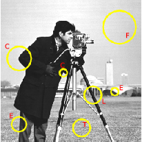
Fig. 6.1 Local Structure in images. In an image we distinguish several types of local structure like constant patches (F), edges (E), lines (L), corners (C) etc.

Note that the local structure patches in the image are of different size. This is inevitable for any visual perception system looking at the 3D world. Objects that are further from the camera (or the eye for the human visual system) are depicted with smaller size in the image. In case there is no a priori knowledge about the size (or scale) of the image details we are interested in, we need to analyze an image at all scales.

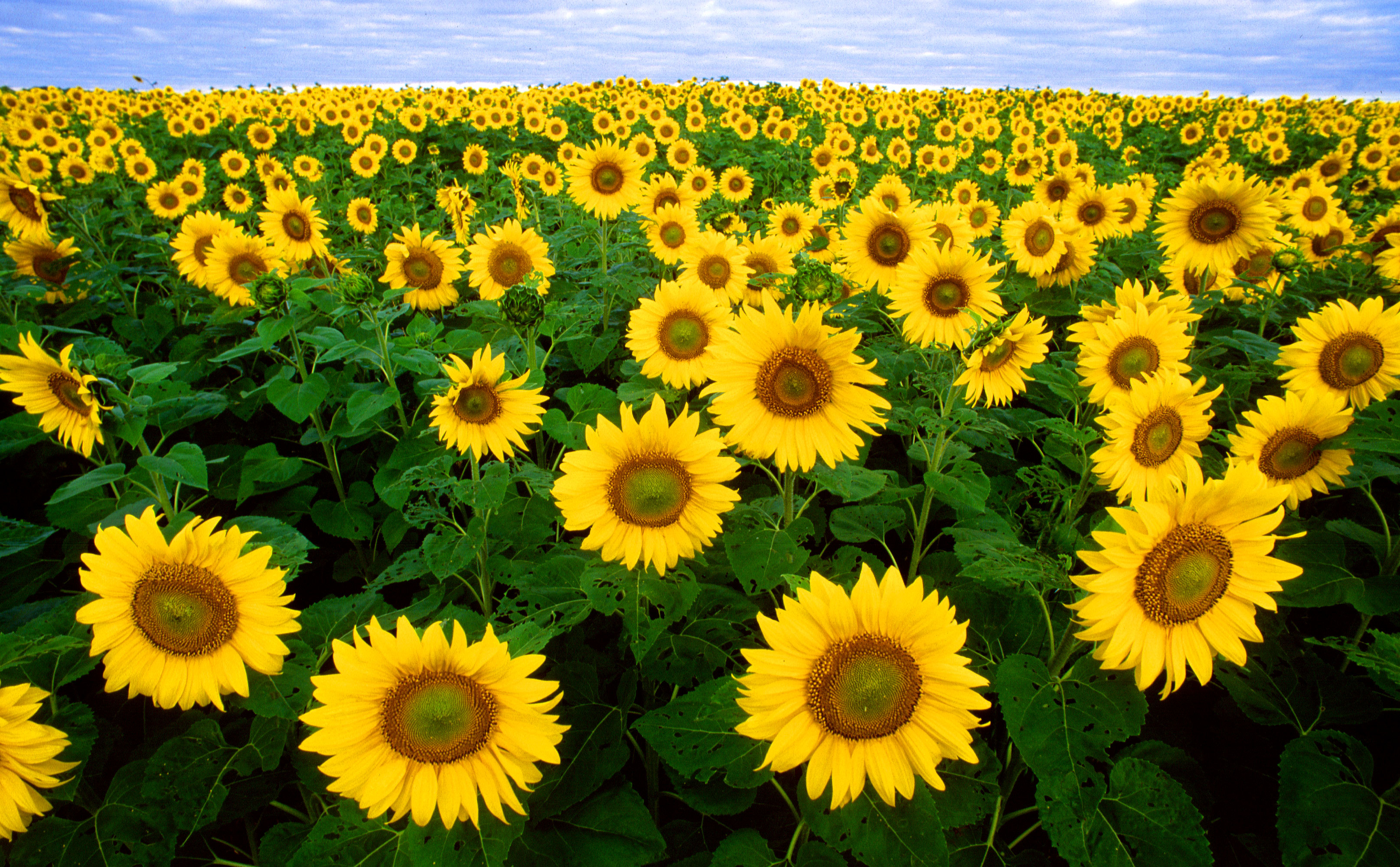
Fig. 6.2 A field of sunflowers.

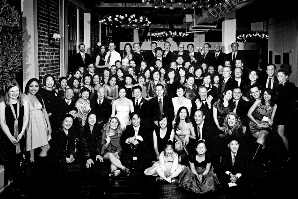
Fig. 6.3 A large group portrait.

In both Fig. 6.2 and Fig. 6.3 3D objects of (almost) constant size are depicted. Sunflowers in the first image and human heads in the second image. The size of the sun flowers and the heads vary in the images due to the ‘divide-by-depth’ phenomenon: objects further from the camera are depicted smaller in an image.

When quantifying local structure in images we thus need to define:

• the notion of local, and
• the notion of structure.

First we introduce the Gaussian linear smoothing as the way to ‘select’ the ‘scale’ (size) of the local neighborhood, then we we will consider derivatives as the mathematical way to characterize local changes in the image function.

The coordinates \(x,y\) in the image function \(f(x,y)\) are arbitrary: if you rotate the camera a bit, or even put it upside down, the values \(f(x,y)\) change but the pictorial content will be more or less the same. So calculating partial derivatives in \(x\) and \(y\) directions seems of little use to describe local changes in the image.

In the section on local structure we will introduce local coordinate systems such that for every point in the image the coordinate axes are aligned with the image contents. In that way rotating your camera (and thereby changing the global \(x\) and \(y\) coordinates) does not influence the local changes with respect to the local coordinates.

There is no unique local coordinate system that works in all situations. In this chapter we will consider two such local coordinate systems: the gradient system and the curvature system.

• 6.1. Gaussian Smoothing and Gaussian Derivatives
  • 6.1.1. Properties of the Gaussian Convolution
  • 6.1.2. Calculating Derivatives of Sampled Functions
  • 6.1.3. Algorithms for Gaussian Convolutions
• 6.2. Local Structure

Extra reading material:

• A gentle introduction to Local Structure in Scale Space for a general overview,
• the slides as a reference of what has been discussed in the lectures, and
• chapter 6 from the 'old' lecture notes

Also consider:

• 6.3. Canny Edge Detector
  • 6.3.1. Edges in 1D
  • 6.3.2. Edges in 2D
• 6.4. Subpixel Localization of Local Structure
  • 6.4.1. Isophotes — Contour Lines
  • 6.4.2. Edges
  • 6.4.3. Lines
  • 6.4.4. X-Corners
  • 6.4.5. Concluding (computational) remarks

The Canny edge detector is obligatory in this course, subpixel localization is not.