6.4. Subpixel Localization of Local Structure

Image data is measured only in the sample points. You may think that because of this we can also localize the structure in images only with pixel distance accuracy. This is not the case fortunately. We can determine the location of local structure with sub pixel accuracy in many cases.

The ability to localize local structure at subpixel accuracy is important in several practical applications:

• Finding characteristic points in an image based on a local structure description is dependent on the accurate localization of those points. E.g. in the SIFT procedure the extrema in \(\ell(\v x,s)=s^2( f\ast \nabla^2 G^s)(\v x)\) (the scale normalized Laplacian) are calculated with subpixel accuracy much the same way as done in this section.
• In calibrating camera’s and when reconstructing the 3D structure from several 2D views of the scene, it is extremely important to localize points in images with great accuracy. In this section we look at an example to localize X-corners on the block patterns used to calibrate camera’s.
• In medical image processing the same part of the human anatomy (say the head) is often ‘seen’ using several imaging devices (e.g. an X-ray and an MRI scanner). For diagnosis it is important to match these two views such that for one point in the head we are able to determine where in the 3D images this point can be found. This registration of the images needs to be done with subpixel accuracy to make accurate measurements and thus a reliable diagnosis possible.

These are just a few examples where the need for subpixel accurate localization arises. In this section we look at sub pixel accurate localization methods for contour lines (isophotes), edges, lines and X-corners (saddle points).

6.4.1. Isophotes — Contour Lines

Consider the isophote \(f(\v x)=c\) where \(c\) is some constant in the range of the scalar function \(f\). Let \(\partial(\set X)\) be the contour of a set \(\set X\subset\setR^d\) (i.e. the set minus its interior), then the (set of) isophote(s) is given by \(\partial(f\geq c)=\partial(f\leq c)\).

For a discrete image \(F\) (let’s assume that \(F\) is the sampled version of \(f\)) the inner contour \(\partial(F\geq c)\) and the outer contour \(\partial(F\leq c)\) are not equal.

Assume that \(\v a\) is a grid point on either the inner or outer contour. A first order Taylor series approximation along the line from \(\v a\) in the gradient direction \(\v e_w\) then is:

\[f(\v a+w\v e_w)\approx f(\v a)+wf_{w}(\v a)\]

Setting this equal to \(c\) and solving for \(w\) we find the subpixel localization of the contour point:

\[\v a_c = \v a + \frac{c-f(\v a)}{f_w(\v a)}\v e_w\]

In cartesian coordinates:

\[\begin{split}\v a_c = \v a + \frac{c-f(\v a)}{f_x^2(\v a)+f_y^2(\v a)}\matvec{c}{f_x(\v a)\\f_y(\v a)}\end{split}\]

Fig. 6.4 Subpixel Accurate Isophote Localization. In this figure the samples of function \(f(\v x)=A-\|\v x - \v x_0\|^2\) are shown as a grey value image (where \(\v x_0\) is the center of the image and the value of the constant \(A\) is chosen to make the image positive on its entire domain). Three isophotes are shown. In red squares the points on the discrete outer contour are shown and in red dots the corresponding subpixel accurate localization. In green squares and dots the discrete inner contour and its subpixel accurate localization are shown. The curves drawn are the ‘true’ isophote curves.

In the example the scale for the Gaussian differentiation was set at 1. Experiments did indicate that accuracy of the subpixel localization in this case was not much dependent on the scale however.

For the discrete contour (either the inner or the outer contour) it is easy to derive the ordering of the points in such a way that the contour is traversed as a curve, in other words it is easy to ‘connect the dots’. The same ordering of points may be used to order the subpixel accurate localized points on the curve.

The classical algorithm to to find a subpixel accurate contour of sampled data is the marching squares algorithm. The marching squares algorithm is somewhat related to the presented one as it is also based on a first order interpolation scheme. In the marching squares algorithm a list of straight line segments is found representing the contour, circumventing the need to find an explicit ordering of the contour points.

6.4.2. Edges

The Canny edge detector is defined with the two conditions:

\[f_{w}\gg 0,\quad f_{ww}=0\]

i.e. we are looking for points with high gradient norm and being zerocrossings in the second order derivative in the (gradient) \(w\)-direction. Let \(\v a\) be a sample grid point where \(f_{w}\gg0\) and where \(f_{ww}\) changes sign in the local neighborhood (a test to check whether the value of \(f_{ww}\) is close to zero is unwise as its value may wildly fluctuate between sample points).

Fig. 6.5 Subpixel Accurate Canny Edge Detector. The gray value image shows a linear edge. In red diamonds the gridpoints where a zero crossing is found are indicated. The green squares are the subpixel accurate locations of the edge (zerocrossings in the second derivative in the gradient direction.

In a local neighborhood of point \(\v a\) we can approximate \(f\) along a line in the gradient direction with a third order Taylor polynomial:

\[f(\v a+w\hat{\v w})\approx f(\v a)+wf_{w}(\v a)+\half w^{2}f_{ww}(\v a)+\small{\frac{1}{6}}w^{3}f_{www}(\v a)\]

where \(w\) is the coordinate along the line with greyvalues \(g(w)=f(\v a+w\hat{\v w})\). The zero crossing in the second order derivative \(g_{ww}\) thus is \(g''(w)=f_{ww}(\v a)+w f_{www}(\v a)\) leading to a zerocrossing at:

\[w^\star = -\frac{f_{ww}(\v a)}{f_{www}(\v a)}\]

and thus the zero crossing relative to \(\v a\) is found at:

\[\v a_{zc}=\v a-\frac{f_{ww}(\v a)}{f_{www}(\v a)}\hat{\v w}\]

In previous sections we have allready encountered the derivatives up to order 3 in the \(vw\)-coordinate system:

\[\begin{split}\hat{\v w} & = & \frac{\nabla f}{f_{w}}\\ f_{ww} & = & \frac{f_{x}^{2}f_{xx}+2f_{x}f_{y}f_{xy}+f_{y}^{2}f_{yy}}{f_{w}^{2}}\\ f_{www} & = & \frac{f_{x}^{3}f_{xxx}+3f_{x}^{2}f_{y}f_{xxy}+ 3f_{x}f_{y}^{2}f_{xyy}+f_{y}^{3}f_{yyy}}{f_{w}^{3}}\end{split}\]

Substitution into the expression for \(\v a_{zc}\) leads to:

\[\begin{split}\v a_{zc}=\v a-\frac{f_{x}^{2}f_{xx}+2f_{x}f_{y}f_{xy}+ f_{y}^{2}f_{yy}}{f_{x}^{3}f_{xxx}+3f_{x}^{2}f_{y}f_{xxy}+3f_{x}f_{y}^{2}f_{xyy}+ f_{y}^{3}f_{yyy}} \matvec{c}{f_x\\f_y}\end{split}\]

6.4.3. Lines

The line detector defined in the 2nd order curvature gauge system is:

\[f_{pp}\approx0,\quad f_{qq}\geq\epsilon\]

Fig. 6.6 Subpixel Accurate Line Detection. The red diamonds indicatie the grid points selected by the line detector. The green squares indicate the subpixel line positions.

The above conditions define bright lines on a dark background. Along the line the curvature is small (the \(\v p\)-direction) and across the line (the \(\v q\)-direction) the curvature is high. To reverse the contrast the role of \(p\) and \(q\) should be interchanged. To locate the midpoint of the line at subpixel accuracy we need to find an analytical description of the luminance function \(f\) in the \(\hat{\v q}\) direction (i.e.perpendicular to the line). The Taylor series expansion is:

\[f(\v a+q\hat{\v q})\approx f(\v a)+qf_{q}(\v a)+\half q^{2}f_{qq}(\v a)\]

The line midpoint is characterized as the local maximum in the \(\hat{\v q}\)-direction, i.e.\(f_{q}=0\). From the above:

\[f_{q}(\v a+q\hat{\v q})\approx f_{q}(\v a)+qf_{qq}(\v a)\]

Setting this equal to zero and solving for \(q\) results in the midpoint:

\[\v a_{mp}=\v a-\frac{f_{q}}{f_{qq}}\hat{\v q}\]

We leave it as an exercise to derive the subpixel line localization in cartesian coordinates.

6.4.4. X-Corners

An X-Corner is what you see on checkerboards. Two bright squares meeting in a corner on a dark background. When we observe the local structure of an X-corner using Gaussian derivatives at scale \(s\), we `see’ a saddlepoint at the corner position.

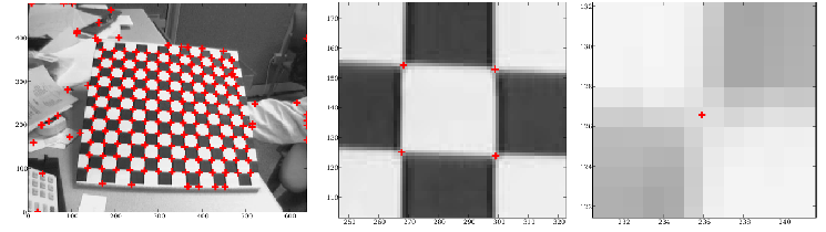
Fig. 6.7 Subpixel Accurate Corner Detection. On the left the image of the checkerboard pattern used for calibration with all detected saddle points marked with crosses. The two images on the right show a detail from the image on the left in order to show the subpixel localization.

A saddlepoint is where the principal curvatures are of opposite signs. That is, we are looking for the points where:

\[f_{x}=f_{y}=0,\quad f_{pp}f_{qq}<0\]

Locally around point \(\v a\) we can write the luminance function as:

\[f(\v a+\v x)\approx f(\v a)+\v x\T(\nabla f)(\v a)+\half\v x\T\v H_{f}(\v a)\v x\]

Let \(\v a\) be a candidate (sampling grid) point where \(f_{pp}(\v a)f_{qq}(\v a)<0\) then we may search for the saddle point location in the neighborhood of \(\v a\) by looking at the point \(\v x\) where the gradient of the above Taylor polynomial vanashish:

\[(\nabla f)(\v a)+\v x\T\v H_{f}(\v a)=0\]

Solving for \(\v x\) we find the sub pixel accurate estimate of the X-corner:

\[\v a_{\mbox{X}}=\v a-\v H_{f}\inv(\v a)(\nabla f)(\v a)\]

6.4.5. Concluding (computational) remarks

In the preceding subsections we have been looking at the location of an \(n\)-th order extremum (zero order for the isophote, second order for the edge, first order for the line and again first order for the X-corner) and in all cases we needed an \((n+1)\)-th order Taylor approximation in a local neighborhood of the extremum.

In all examples it was possible to select candidate sample points (say the point \(\v a\)). For each of these candidate points we calculated the \((n+1)\)-th Gaussian jet and from that the subpixel deviation \(\Delta \v a\) leading to the subpixel accurate location \(\v a + \Delta \v a\). In all examples we have used a very simple test to see whether the resulting estimate was correct. Assuming a unit square sampling grid we accept the subpixel estimate in case \(\|\Delta \v a\|_\infty<\half\), i.e.the estimate is accepted in case the subpixel location is close to \(\v a\) (“lies within the pixel corresponding with sample point \(\v a\)“). If this is not the case we expect that there will be another grid point \(\v a'\) that is closer to the subpixel estimate.