6.1. Gaussian Smoothing and Gaussian Derivatives
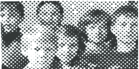
\(f\ast G^{1}\)
\(f\ast G^{3}\)
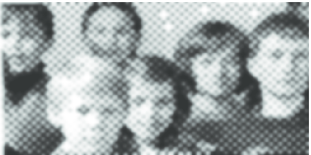
\(f\ast G^{7}\)

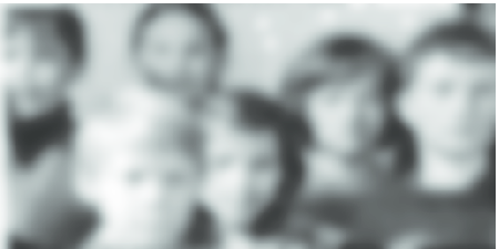
\(f\ast G^{11}\)
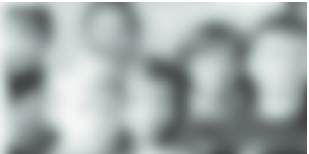
\(f\ast G^{13}\)
Consider an image of a photo printed in a newspaper. Because the image is depicted at larger size then it was printed in the newspaper, the individual blobs of ink are visible. In black and white printing only black ink is used, the ‘illusion’ of gray tones is due to the fact that the human eye cannot resolve too small details. We could say that the human eye is smoothing the images.
We can do the smoothing with the computer. In the next figure we show a sequence of images all of which are local mean filtered versions of the news paper image. The smoothing (local mean) is done using a Gaussian weight function.
A smoothed function is the convolution of the orginal function \(f\) with the Gaussian weight function \(G^s\):
The size of the local neighborhood is determined by the scale of the Gaussian weight function.
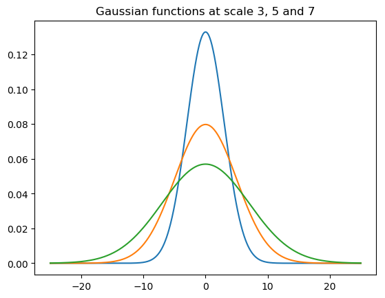
In the plot three 1D Gaussian functions are shown for scales 3, 5 and 7. The graph of the 2D Gaussian function is obtained by rotating the 1D function graphs around the vertical \(z\)-axis.
6.1.1. Properties of the Gaussian Convolution
The Gaussian kernel function used in a convolution has some very nice properties.
Separability
The property that is of great importance in practice is that is a separable function in the sense that we may write:
where \(G^s(x)\) and \(G^s(y)\) are Gaussian functions in one variable:
It is not hard to prove (starting from the definition of the convolution) that a separable kernel function leads to a separable convolution in the sense that we may first convolve along the rows with a one dimensional kernel function followed by a convolution along the columns of the image. The advantage is that for every pixel in the resulting image we have to consider far less values in the weighted sum then we would have to for a straightforward implementation.
Semi Group
If we take a Gaussian function \(G^s\) and convolve it with another Gaussian function \(G^t\) the result is a third Gaussian function:
Mathematicians refer to such a property with the term semi group (it would be a group in case there would be an ‘inverse Gaussian convolution’).
From a practical point of view this is an important property as it allows the scale space to be build incrementally, i.e. we don’t have to run the convolution \(f_0\ast G^s\) for all values of \(s\). Say we have already calculated \(f^t = f_0\ast G^t\) (with \(t<s\)), then using the associativity and the above property we have:
Note that \(\sqrt{s^2-t^2}<s\) and thus the above convolution will be faster then the convolution \(f_0\ast G^s\).
Smoothness and Differentiability
Let \(f_0\) be the ‘original’ image and let \(f^s\) be any image from the scale space (with \(s>0\)). Then no matter what function \(f_0\) is, the convolution with \(G^s\) will make into a function that is continuous and infinitely differentiable. Using Gaussian convolutions to construct a scale space thus safely allows us to use many of the mathematical tools we need (like differentation when we look at the characterization of local structure).
6.1.2. Calculating Derivatives of Sampled Functions
Building a model for local image structure based on calculating derivatives was considered a dangerous thing to do in the early days of image processing. And indeed derivatives are notoriously difficult to estimate for sampled functions. Remember the definition of the first order derivative of a function \(f\) in one variable:
Calculating a derivative requires a limit where the distance between two points (\(x\) and \(x+dx\) is made smaller and smaller. This of course is not possible directly when we look at sampled images. We then have to use interpolation techniques to come up with an analytical function that fits the samples and whose derivative can be calculated.
Let \(F\) be a sampled image then we may calculate the first order derivative \(F_x\) as:
or with:
or with:
Note that all these ‘derivative images’ are only approximations of the sampling of \(f_x\). They all have their role in numerical math. The first one is the right difference, the second the left difference and the third the central difference.
In these lecture notes we combine the smoothing, i.e. convolution with a Gaussian function, and taking the derivative. Let \(\partial\) denote any derivative we want to calculate of the smoothed image: \(\partial(f\ast G^s)\). We may write:
Even if the image \(f\) is a sampled image, say \(F\) then we can sample \(\partial G^s\) and use that as a convolution kernel in a discrete convolution.
Note that the Gaussian function has a value greater than zero on its entire domain. Thus in the convolution sum we theoretically have to use all values in the entire image to calculate the result in every point. This would make for a very slow convolution operator. Fortunately the exponential function for negative arguments approaches zero very quickly and thus we may truncate the function for points far from the origin. It is customary to choose a truncation point at about \(3s\).
Note that because \(G^s\) is separable, \(\partial G^s\) is separable as well. This allows for separable convolution algorithms for all Gaussian derivatives.
6.1.3. Algorithms for Gaussian Convolutions
There are several ways to implement the Gaussian (derivative) convolutions to work on sampled images:
Straightforward implementation. This is the direct implementation of the definition of the discrete convolution using the fact that the Gaussian function is seperable and thus the 2D convolution can be implemented by first convolving the image along the rows followed by a convolution along the columns.
In this straightforward implementation the Gaussian function is sampled on the same grid as the image to be convolved. Although the Gaussian function has an unbounded support (i.e. \(G^s(x)>0\) for all \(x\)) we may ‘cut-off’ the sampled version for values of \(|x|>t\). The value of \(t\) is scale dependent! (this is part of the Lab Exercises).
It should be evident that for small scale values this straightforward implementation will not be accurate. For, say, \(s<1\) the Gaussian function is restricted to only a few pixels. Such a ‘small’ Gaussian function is really not suited to be sampled on the grid with \(\Delta x\).
Interpolated Convolution. Instead of bluntly sampling the Gaussian function and calculate the discrete convolution we could first interpolate the discrete image, then calculate the convolution integral and finally sample to obtain the discrete image (this is detailed in the section “From Convolution Integrals to Convolution Sums” in the previous chapter). The interpolated convolution turns out to be equivalent with a discrete convolution with a weight function that is slightly different from the Gaussian (derivative) weight function.
Convolution using the Fast Fourier Transform. In we first calculate the Fourier Transform of the input image and the convolution kernel the convolution becomes a point wise multiplication. Let the input image be of size \(N\times N\) the spatial implementation is of order \(O(N^2)\) whereas the FFT version is \(O(N\log N)\). This may seem like an important speed up, still the spatial implementation are nowadays more often used.
Infinite Response Convolution. These are probably the fastest implementations. The gain in speed is obtained because the local neighborhood used is of the same size regardless of the scale of the Gaussian function. Disadvantage of this method is that it is only an approximation and that calculating Gaussian derivatives is troublesome.