1. Images
An image is a mathematical representation of a physical observation as a function over a spatial domain. At every point on the retina (the photosensitive surface in the eye or camera) the electromagnetic energy is measured. For a computer scientist the physical laws that govern image formation and image observation are just that: laws. We can’t change them; we have to live with them. Needless to say that this does not mean that we need not familiarize ourselves with these physical laws. It is senseless to develop programs that are not in accordance with physical reality. Especially in the field of machine vision the physical (and psycho-physical) description of the sensors is the starting point in utilizing these sensor signals in information systems. Therefore we would like to treat an image as defined over a continuous spatial domain, not as a mere collection of pixel values. The fact that we need to discretize an image by sampling should be considered a practical inconvenience that should be banned from our thinking once we have dealt with the matter in the very beginning. Only on the lowest level in an image information system should we be concerned with the fact that the individual pixels make up the discrete representation of the image. Most of our image processing work and image analysis work should regard images as mappings over a continuous domain and treat them accordingly. For a computer scientist this might seem a rather awkward and counterintuitive starting point. He or she is probably familiar with images being large arrays of say \(800\times 600\) pixels, each representing a color specified as an RGB triplet.
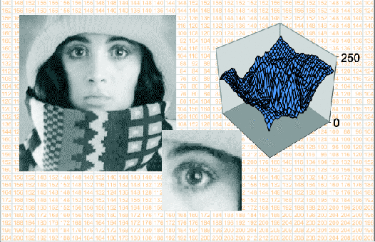
Fig. 1.11 Images. The image on the left and the small detail of the eye are ‘real’ images to our eye. The two dimensional function surface in the top right carries the same information as the image depicting the eye. In this case however the luminance value corresponds with the vertical height of the functions surface. The array of numbers is a detail of the larger array of numbers that is really represented in the computer.
Fig. 1.11 above illustrates the difference between what the human visual brain perceives as an image (the photograph), its mathematical model (the image function visualized as the luminance surface) and its discrete representation (the array of numbers). In this chapter we will develop the mathematical tools to think in terms of the mathematical model (the image function) when only the image samples (the array of numbers) are given.
In this chapter we look at:
- Image Formation: The optical formation of images is briefly discussed.
- Image Definition: Images as mappings from a continuous domain (most often 2D space) to the set of real numbers (most often the luminance measurements).
- Image Discretization: A pixel is not a little square such that all pixels in an image ‘tile’ the image domain, a pixel is the outcome of the measurement of electromagnetic wave energy in a small (but not infinitessimally small) spot on the retina (either in the human eye or in a camera). A discrete image is a sampled and quantized version of the spatial distribution of the electromagnetic energy.
- Image Interpolation: whereas sampling takes us from a function defined on a continuous domain to a set of samples, interpolation does the opposite. Given a set of samples (like a discrete image) it generates a function defined on the continuous domain. It is seldomly true that sampling and interpolation are truly inverse operators.
- Image Representation: a digital image can be represented as an array of all image samples. This section hopefully sheds some light on the confusion between the different choices to be made for coordinate axes and indices.