1.6. Image Histograms

1.6.1. Univariate Histogram

A histogram of all possible scalar pixel values in an image provides a summary of the distribution of the values over all possibe values:

\[h_f[i] = \sum_{\v x\in E} \left[ e_i \leq f(\v x) < e_{i+1} \right]\]

where \([ \text{condition}]\) is 1 in case the condition is true and zero otherwise. Here \(e_i\) for \(i=0,\ldots,n\) are the bin edges in the histogram. The histogram value \(h_f[i]\) is calculated for \(i=0,\ldots,n-1\). The formula above is what the histogram function from numpy is calculating. Please read the documentation to read in what way you can determine the number of bins and the bin edges that are being used.

Observe carefully that the histogram function automagically chooses \(e_0\) to be equal to the minimal value of \(f\) and \(e_1\) to be equal to the maximal value. In most cases that is ok, but in case you want to compare histograms of several images you better choose your bin edges equal accross all images.

1.6.2. Multivariate Histograms

Now assume your data to be histogrammed is n-dimensional, e.g. a color image where \(n=3\). You could make univariate histograms of the three colors R, G and B but then the correlation of the colors is not captured in the histogram. It is best to make a real three dimensional histogram with three dimensional bins. Every bin this is a rectangular 3D volume. Let \(\v f(\v x)\) be a color image:

\[\begin{split}\v f(\v x) = \matvec{ccc}{f_1(\v x)\\ f_2(\v x)\\ f_3(\v x)} = \matvec{ccc}{r(\v x)\\ g(\v x)\\ b(\v x)}\end{split}\]

The histogram then is:

\[h_f[i,j,k] = \sum_{\v x \in E} \left[ e_{1,i} \leq f_1(\v x) < e_{1,i+1} \right] \left[ e_{2,j} \leq f_2(\v x) < e_{2,j+1} \right] \left[ e_{3,k} \leq f_3(\v x) < e_{3,k+1} \right]\]

The product of the ‘condition brackets’ is one only in case \(\v f(\v x)\) is within the 3D bin with indices \((i,j,k)\).

A multivariate histogram can be calculated with the histogramdd function from numpy. Evidently visualizing a 3D (or even higher dimensional) histogram is not a trivial task. Here we give a very simple way to do so. [1]

def histogram3dplot(h, e, fig=None):
    """
    Visualize a 3D histogram

    Parameters
    ----------

    h: histogram array of shape (M,N,O)
    e: list of bin edge arrays (for R, G and B)
    """
    M, N, O = h.shape
    idxR = np.arange(M)
    idxG = np.arange(N)
    idxB = np.arange(O)

    R, G, B = np.meshgrid(idxR, idxG, idxB)
    a = np.diff(e[0])[0]
    b = a/2
    R = a * R + b

    a = np.diff(e[1])[0]
    b = a/2
    G = a * G + b

    a = np.diff(e[2])[0]
    b = a/2
    B = a * B + b

    colors = np.vstack((R.flatten(), G.flatten(), B.flatten())).T/255
    h = h / np.sum(h)
    if fig is not None:
        f = plt.figure(fig)
    else:
        f = plt.gcf()
    ax = f.add_subplot(111, projection='3d')     
    mxbins = np.array([M,N,O]).max()
    ax.scatter(R.flatten(), G.flatten(), B.flatten(), s=h.flatten()*(256/mxbins)**3/2, c=colors)

    ax.set_xlabel('Red')
    ax.set_ylabel('Green')
    ax.set_zlabel('Blue')

In [1]: from scipy.ndimage import imread

In [2]: from ipcv.ip.histogram3dplot import histogram3dplot;

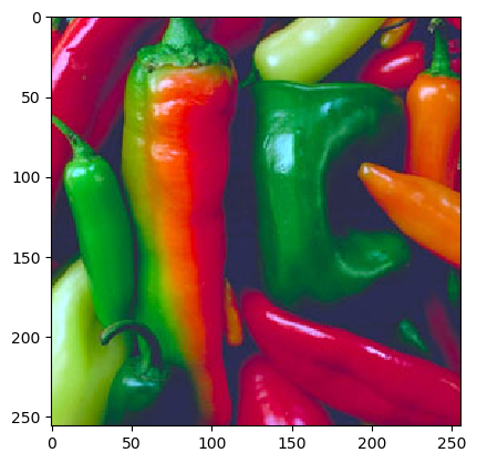
In [3]: f = imread('python/data/images/peppers.png')

In [4]: plt.figure(1);

In [5]: plt.imshow(f);

In [6]: h, e = np.histogramdd(f.reshape(-1,3), bins=8)

In [7]: histogram3dplot(h, e)

In [8]: plt.show();

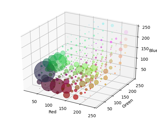
In the above 3D histogram display the histogram is 8x8x8 bins. The bins are 3D cubes. At the RBG position of each bin we display a disk like marker in the color corresponding with the color in the RGB spae and with a radias that is proportional to histogram count.

The histogram visualization shows that there are a lot of reddish and greenish pixels in the image and that there are a lot of dark blueish pixels (the darker spots in between the peppers).

When you run the program yourself you can rotate the plot by clicking a dragging. Then it is easier to see the distribution of colors in the RGB cube.

Visualizing a 2D histogram is much easier: \(h_f[i,j]\) can be visualized as a scalar image. Numpy has a function histogram2d just for 2D data: please read the documentation carefully.

Footnotes

[1]

It would be much nicer to have a color histogram visualization where the ‘markers’ are really 3D markers. For instance cubes of the color corresponding with its position in the RGB cube and a size proportional to the number of counts. An implementation in OpenGL would be best of course. Any volunteers?