1.4. Image Interpolation
Given the samples \(F\) of an image \(f\) the task of interpolation is to calculate a value for \(f(x,y)\) even for those \((x,y)\) that are not sample points.
In most cases it is not realistic to ask for the value \(f(x, y)\): a unique value only exists in case the sampling proces is without loss of information. For band-limited images indeed such a unique interpolated function exists, because ideal bandlimited images (functions) can be sampled without loss and thus can be reconstructed without error. [#fn_bandlimited]_
In these lecture notes we start from a rather pragmatic point of view. We assume that the digital images we start with are oversampled i.e. the samples are close enough to eachother to faithfully represent the image \(f\). Surely we have to take care not to undersample images in our computational analysis without presmoothing as we would be computationally introducing aliasing then.
In this section we start with interpolation for 1D functions, that is we start with interpolation of sampled univariate functions. We will discuss only a few techniques that are commonly used. Then we show how to generalize these 1D interpolation methods to 2D (and nD if needed).
1.4.1. Interpolating 1D functions
Consider the samples \(F(k)\) of a function \(f(x)\). We assume that the sampling interval is 1, i.e. \(F(k)=f(k)\). The goal of interpolation is to find an estimate of \(f(x)\) for arbitrary \(x\) given only the sampled (discrete) function \(F\).
1.4.1.1. Nearest neighbor interpolation
Nearest neighbor interpolation is the simplest interpolation method. Given the samples \(F(k)\) the value of the interpolated function \(\hat f\) at coordinate \(x\) is given as:
i.e. we simply select the sample point that is nearest to \(x\). Here \(\lfloor x \rfloor\) is the floor function, i.e. the largest integer values that is less then or equal to \(x\).
This leads to a staircase type of interpolated function. The function \(\hat f\) is indeed defined on the entire real axis but it is neither continuous (as it contains jumps) nor differentiable.
As an example we look at the function \(f(x)=sin(x)\) and its nearest neighbor interpolated version.
In [1]: from scipy.interpolate import interp1d

In [2]: x = np.linspace(0, 6, 200); # fine sampling to represent continuous function

In [3]: xs = np.array([0, 1, 2, 3, 4, 5, 6]); # the sample points

In [4]: f = np.sin(x); F = np.sin(xs); # the 'continuous' function and its sampled version

In [5]: ifunc = interp1d(xs, F, kind='nearest'); hatf_nn = ifunc(x);

In [6]: plt.clf(); plt.plot(x, f, 'g-', xs, F, 'ro', x, hatf_nn, 'b-');
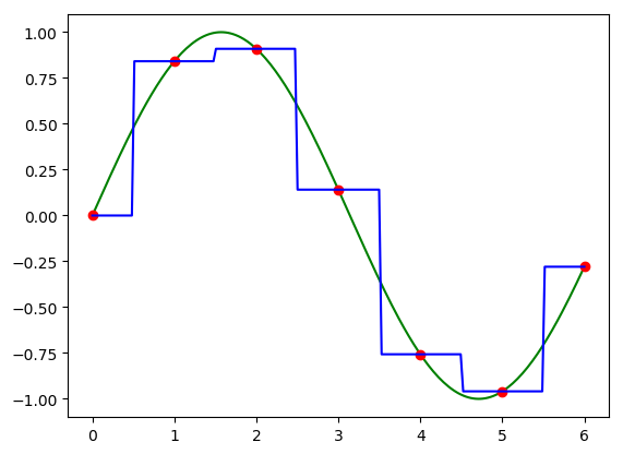
In green the continuous function \(f\) (note that we did sample this function too… but we did so with a very small sample width and thus for our eye the plot looks like a continuous function), in red the sampled function and in blue the interpolated function.
1.4.1.2. Linear Interpolation
Linear interpolation is the scientific equivalent of what you have already learned in kindergarten: connect the dots. Between to adjacent sample points \(k\) and \(k+1\) we assume the function is a linear function and thus in this interval \([k,k+1]\) we have:
In [7]: ifunc = interp1d(xs, F, kind='linear'); hatf_lin = ifunc(x);

In [8]: plt.clf(); plt.plot(x, f, 'g-', xs, F, 'ro', x, hatf_lin, 'b-');
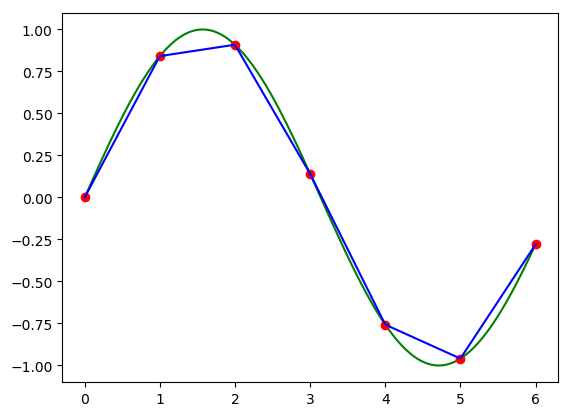
The linearly interpolated function is continuous but it is not everywhere differentiable (in de sample points it’s not differentiable). Furthermore for the interpolated function the second and higher order derivatives are equal zero (except for the sample points where these are not defined).
Although a simple interpolation method, linear interpolation is very often used in practice. It is simple to implement and very fast.
1.4.1.3. Cubic Interpolation
In nearest neighbor interpolation only one sample is used (the nearest) to set the interpolated value. In linear interpolation we look at the 2 closest sample points (one on the left and one on the right). For cubic interpolation we look at two pixels on the left and two on the right.
To interpolate between \(x=k\) and \(x=k+1\) we fit a cubic polynomial
to the 4 sample points \(k-1, k, k+1\) and \(k+2\). For the 4 points we have:
Solving these equations for \(a,b,c\) and \(d\) we get:
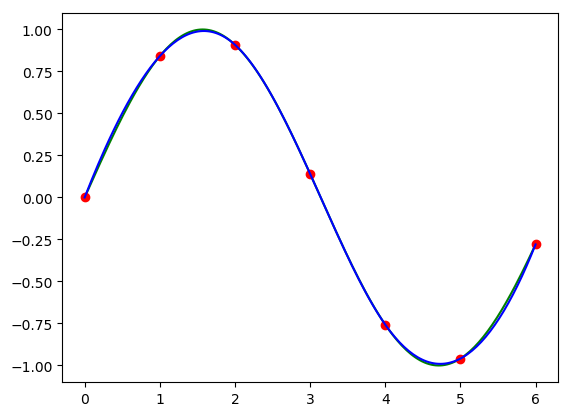
In [9]: ifunc = interp1d(xs, F, kind='cubic'); hatf_cubic = ifunc(x);

In [10]: plt.clf(); plt.plot(x, f, 'g-', xs, F, 'ro', x, hatf_cubic, 'b-');
1.4.1.4. Even Better Interpolation
There are even better interpolation methods to be used. A straightforward generalization would be to consider even more samples to estimate the function value of \(f\). Taking \(n\) samples to the left of \(x\) and \(n\) samples to the right we need a polynomial of order \(2n-1\). A big disadvantage of higher order polynomials is overfitting of the original function: higher order polnomials tend to fluctuate wildly inbetween the sample points.
In [11]: xs = np.arange(-7, 8)

In [12]: F = 1.0 * (np.abs(xs) < 3)

In [13]: plt.plot(xs, F, 'o');

In [14]: x = np.linspace(-7, 7, 1000)

In [15]: ifunc = interp1d(xs, F, kind='cubic'); hat_f = ifunc(x)

In [16]: plt.plot(x, hat_f);

In [17]: plt.show()
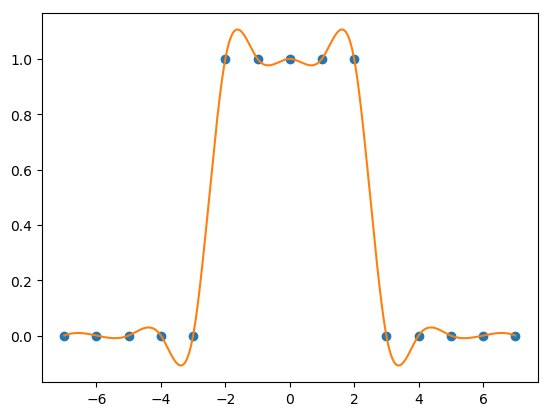
Another disadvantage of the interpolation schemes discussed so far is that the piecewise interpolated function \(\hat f\) shows discontinuities at the sample point positions. This disadvantage can be tackled with spline interpolation.
1.4.2. Interpolating 2D functions
Given an interpolation method for 1D (scalar) functions it is always possible to generalize the method to work with 2D functions (and even higher dimensional ones). As an example consider the linear interpolation. To estimate a value \(f(x,y)\) with \(i\leq x\leq i+1\) and \(j\leq y\leq j+1\) we first interpolate in the ‘\(x\)-direction’ to find values \(f(x,j)\) and \(f(x,j+1)\) and then interpolate in the ‘\(y\)-direction’ to find \(f(x,y)\).
Assume that \(x=i+a\) and \(y=j+b\) (with \(a\) and \(b\) in the interval \([0,1]\)) then:
When generalizing cubic interpolation to two dimensions we need 16 samples in the image (a \(4\times4\) subgrid).
For 2D functions we can also use spline interpolation.