1.2. Image Definition

An image \(f\) is a mapping from a spatial domain \(E\) to a range \(V\), i.e. \(f: E \rightarrow V\) and thus each element \(\v x\in E\) is mapped onto a value \(f(\v x)\in V\), i.e. \(\v x\in E \mapsto f(\v x) \in V\).

The domain of an image is the continuous Euclidean space (in principle we may position the image samples at all points in space): \(E=\setR^d\). In these lecture notes we do not restrict the notion of images to the 2D representation of visual observations only. The measurements as function of 3D space as acquired with a confocal microscope or a medical CT scanner are images as well.

The choice for a basis in that space (and with it a coordinate frame) is arbitrary. For example take two images with your mobile phone where you just slightly change the rotation of the camera. The natural image coordinate axes (used to index the pixels) will be different whereas the images will show the same scene.

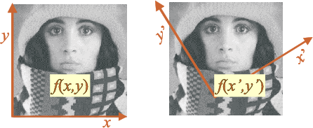
Fig. 1.17 Coordinate Frame. The choice for a basis (and consequently a coordinate frame) is arbitrary.

In these notes we will restrict ourselves mostly to 2D images where the domain is the 2D Euclidean plane \(E=\setR^2\). We will consider many different types of ranges:

Color Images:

For a color image at every point \(\v x\in \setR^2\) we measure three values: the red, green and blue intensity values. The image can be represented as a vector valued function:

\[\begin{split}\v x\in \setR^2 \mapsto \v f(\v x) = \matvec{c}{r(\v x)\\ g(\v x) \\ b(\v x)} \in \setR^3\end{split}\]

Scalar (Grey Value) Images:

An X-ray image is a scalar (grey value) image. At every \(\v x\in \setR^2\) the intensity of radiation is measured. An X-ray image this is a function

\[\v x\in\setR^2 \mapsto f(\v x)\in\setR\]

Often when processing color images we actually only process the intensity value of the color image (i.e. we first turn it into a black-and-white image).

In image processing we start off with an image that is obtained with some physical sensor (a standard camera, or an X-ray camera, etc). In that case the range is \(\setR^+\) as energy measurements will be positive. Image processing algoritms will calculate new images from the original ones. The calculated images (like a derivative of the function \(f(\v x)\)) can be scalar images with a range including the negative numbers.

Indicator (Label) Images:

The goal of a lot of image processing and computer vision tasks is to label the positions in an image domain to belong to a particular class of objects. For example let \(\v f(\v x)\) be a color image depicting people. A image processing task might be to identify all \(\v x\) depicting the human skin. We could then define an image

\[\begin{split}g(\v x) = \begin{cases} 1 &: \v x\in\text{skin region}\\ 0 &: \v x\not\in\text{skin region} \end{cases}\end{split}\]

The binary valued label images form a traditionally important class of images: the binary images.

You could also come up with a label image with more than two possible values, e.g. \(1\): grass, \(2\) road, \(3\) pedestrian, \(4\) building, etc (for an image processing system used in automated vehicles).

A label image is often the outcome of an image analysis procedure that assigns to each point in the image domain the label indicating the semantic class the point belongs to.

What type of image processing is appropriate for an image strongly depends on what type of image it is. Calculating a local average of image values is perfectly reasonable for a color or grey value image but it is questionable for a label image (what should be the meaning of the average of some grass and building label values?).