7. Scale Space
Most of the images we (or computers) look at are taken with optical camera’s projecting our 3D world onto a 2D light sensitive plane (the retina for human eyes or the CCD or CMOS pixel plane for camera’s). We are all familiar with the fact that distant objects are projected at smaller size. The human visual system thus has little a priori knowledge about the scale/size an object will appear on the image.
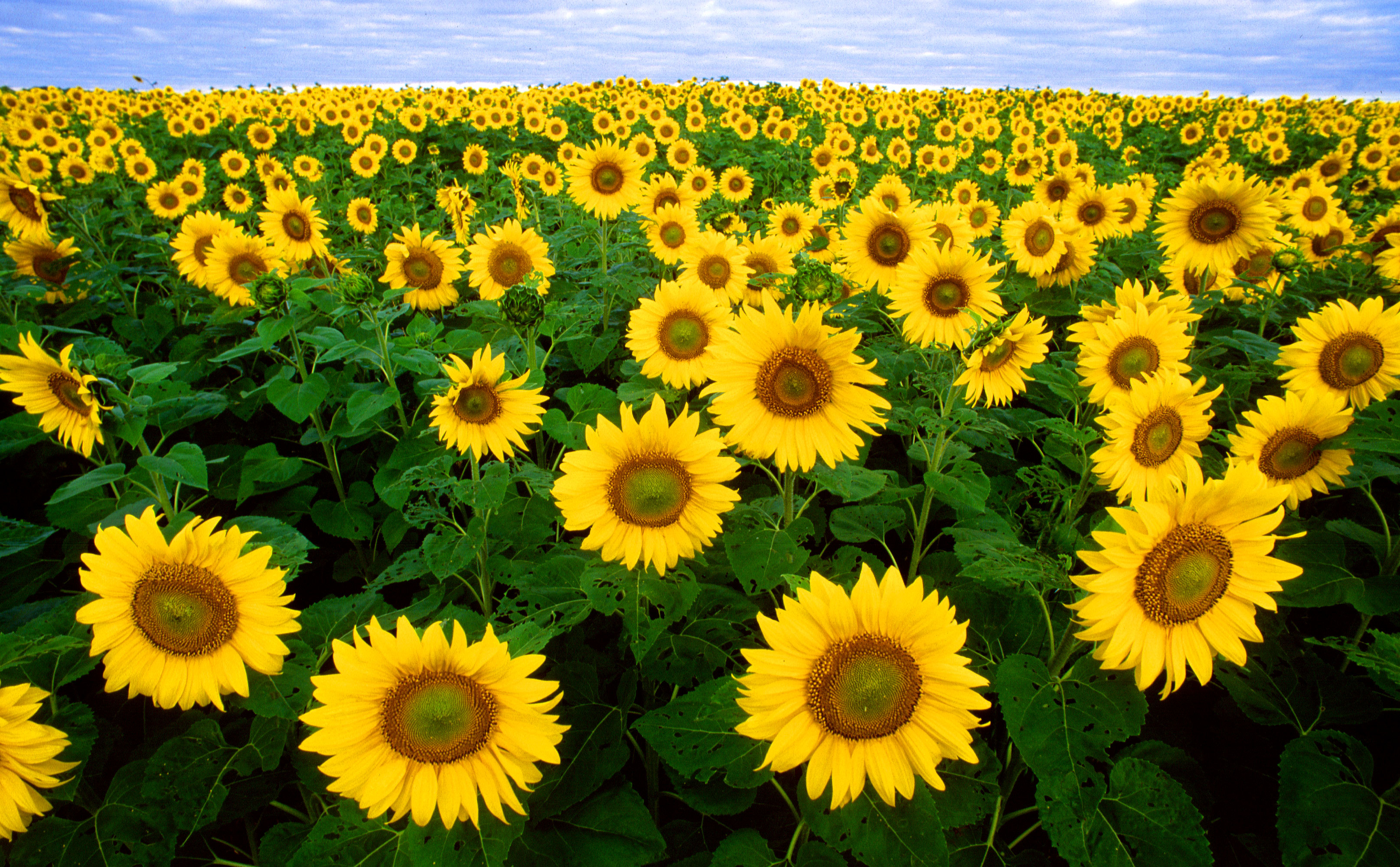
Fig. 7.1 Sunflowers. The size (scale) of the objects is dependent on the distance from the camera. A visual system should be prepared to ‘see’ objects at all possible sizes.
The image in figure Sunflowers is a nice illustration of this effect. The flowers in the front are easily 10 times larger then the flowers near the horizon. Instead of flowers we could equally well look at faces at different distances (and thus size) or at license plates of cars at different distances from the camera.
The only sensible thing to do then is to be prepared for all possible sizes. The image should be processed at all levels of scales simultaneously. In a previous chapter we have already discussed the local structure of images and described that the scale of local details is characterized with the scale of the Gaussian smoothing kernel with which the image is smoothed.
Smoothing an image at all possible scales \(s>0\) leads to what is called a scale-space.
7.1. Definition and Properties
It may seem that there are enumerous ways to construct a scale-space. But surprisingly in case we set some simple requirements there is only one scale-space construction possible.
We are looking for a family of image operators \(\op L^s\) where \(s\) refers to the scale such that given the ‘image at zero scale’ \(f^0\) we can construct the family of images \(\op L^s f^0\) such that:
- \(\op L^s\) is a linear operator,
- \(\op L^s\) is translation invariant (all parts of the image are treated equally, i.e. there is no a priori preferred location),
- \(\op L^s\) is rotational invariant (all directions are treated equally, i.e. there is no a priori preferred direction),
- \(\op L^s\) is separable by dimension, and
- \(\op L^s\) is invariant under change of scale (starting with a scaled version of the zero scale image we should in principal obtain the same scale-space but then offsetted in scale).
Prof. Jan Koenderink from Utrecht University formulated scale-space theory in the 1980’s. The seminal paper is: J.J. Koenderink, The Structure of Images, Biological Cybernetics, 1984. From the abstract:
In practice the relevant details of images exist only over a restricted range of scale. Hence it is important to study the dependence of image structure on the level of resolution. It seems clear enough that visual perception treats images on several levels of resolution
It can be proved that the unique scale space operator satisfying all the requirements is the Gaussian convolution:
where \(G^s\) is the 2D Gaussian kernel:
The function \(f\) can be interpreted as a one parameter family of images. For every scale \(s>0\) there is an image \(f(\cdot,s)\) that we will refer to frequently as \(f^s\).
The scale-space function \(f\) is the solution of the diffusion equation:
with initial condition \(f(\cdot,0)=f^0\). In fact this differential equation was the starting point for Koenderink in deriving linear scale space (see here). From a practical point of view it is an important equation because it tells us that the change in the function \(f\) due to a small change in scale (going from scale \(s\) to scale \(s+ds\)) is proportional to the Laplacian differential structure of \(f\) at scale \(s\). It shows that scale derivatives may always be exchanged for spatial derivatives.
The Gaussian convolution forms a semi-group in the sense that:
This implies that first convolving with a Gaussian at scale \(s\) followed by convolving with a Gaussian at scale \(t\) is equivalent with one convolution at scale \(\sqrt{s^2+t^2}\).
7.2. Scale-Space in Practice
Every slice out of a scale-space can be obtained from the ‘zero-scale’ image by a Gaussian convolution: \(f(\cdot,s) = f_0 \ast G^s\). But what comes out of the camera can’t be the zero scale image. An image at scale \(s=0\) is a mathematical abstraction, observing an image always is at some finite scale (the size of the measurement probe).
The image that comes from the camera often serves as the first image in scale space and assuming \(\Delta x=\Delta y = 1\) a zero scale of \(s_0=\half\) is a common choice (as it results in slightly overlapping probes and thus some smoothness when considering neighboring samples).
To construct the scale space starting at the scale of the observed image (\(s_0\)) we have (for \(s>s_0\)):
7.3. Sampling Scale Space
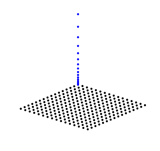
For one slice (the ‘zero-scale’ slice) all the spatial samples are shown, and for one spatial sample (pixel) all the scale samples are shown.
Every ‘slice’ \(f(\cdot,s)\) out of the scale-space is an image and the equidistant sampling is used for all images:
for \(i=0,\ldots,n_x-1\) and \(j=0,\ldots,n_y-1\).
Scale has to be sampled logarithmically:
for \(k=0,\ldots,n_s-1\) (thus \(\log s\) is sampled equidistantly). The need for logarithmic scale sampling becomes clear if you compare \(f\ast G^1\) with \(f\ast G^2\) and also compare \(f\ast G^{11}\) with \(f\ast G^{12}\). For both pairs the absolute increase in scale is the same, however the visual change in smoothing from \(s=1\) to \(s=2\) is much more profound than the change in smoothing from \(s=11\) to \(s=12\).
The consequence of the semi-group property of the Gaussian convolution is that a scale space can be build incrementally. We don’t have to calculate \(f^{s_k}\) by convolving \(f^{s_0}\) we can convolve a previous slice in scale space to obtain the next one:
Note that even for the incremental build of the scale space the scale of the Gaussian kernel grows as the scale increases. Burt’s pyramid discussed in the next section is a way to work with a fixed scale Gaussian kernel.