6.3. Canny Edge Detector

6.3.1. Edges in 1D

In 1D an edge is simple to define. It’s the position (\(x\) value) of the transition from a low value to a high value of the signal (function) or the transition from high to low. In the figure below the canonical edges in a 1D signal are given. What characterizes a point on an edge is:

• its position (\(x\) value)
• the change in function (gray) value across the edge

The mathematical way to express change is by using derivatives. The derivative \(f'(x)\) is proportional to the change in the function value \(f\) when the value of \(x\) is increased slightly.

Consider the canonical edge profile, gradually changing from low to high values. The derivative is almost zero far to the left of the edge, then it gradually increases until it reaches a maximum value (where the edge is) and from there decreases gradually to zero again.

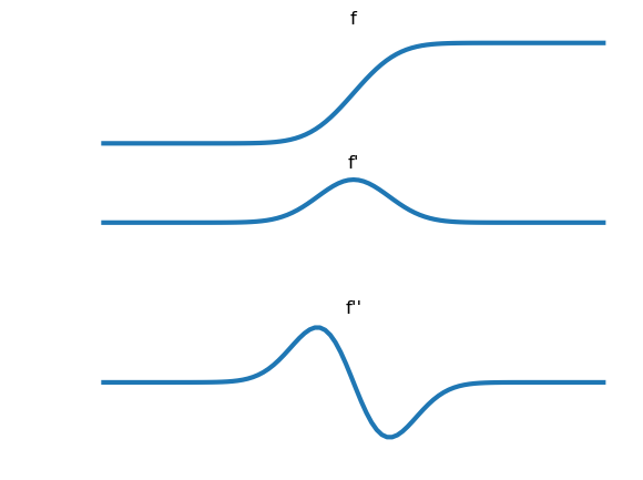
Thus an edge is characterized as a point where the first order derivative (in absolute sense) is large and the second order derivative is almost zero (the change of the first order derivative is minimal):

\[\begin{split}f'(x) \gg 0\\ f''(x) \approx 0\end{split}\]

When implementing such a scheme to work on sampled images we should be careful. The first condition is simple: \(f'(x)\gg 0\) is implemented as a comparison with some threshold \(t\): \(f'(x)>t\). The second condition is troublesome. For course sampled images the second order derivative could change from a relatively large positive value on the left of an edge to a relatively small negative value on the right. Then nowhere near the edge the second order derivative will be equal to zero. We therefore better find a way to check for such zero crossings. We leave that for a Lab Exercise.

6.3.2. Edges in 2D

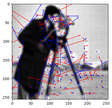
An edge in 2D is most often an edge in 1D where the direction in which to look for the edge can and will differ from point to point in an image. Which direction to choose then? Imagine you are standing on a mountain with a very smooth surface. The height of the surface above sea level (say) can be expressed as a function \(h(x,y)\) (assuming of course that the flat earth assumption is—locally—reasonable). The assumed smoothnes of the function implies that the function can be differentiated.

Standing on that mountain we can turn around at the same spot. In one particular direction we find the mountain is increasing in height maximally. The slope in that direction is the maximal slope of the mountain at that particular point. In the perpendicular direction the slope is zero. That is the direction of the curve of equal height.

Mathematically the direction of maximal slope in a point \(\v a\) is given by the direction of the gradient vector \((\nabla f )(\v a)\):

\[\begin{split}(\nabla f)(\v a) = \matvec{c}{f_x(\v a)\\f_y(\v a)}\end{split}\]

the norm of the gradient vector is equal to the maximal slope.

When looking for edges it is evident to look in the gradient direction. The gradient direction by convention is called the \(w\)-direction and the unit vector in that direction is denoted as \(\v e_w\). The direction perpendicular to the gradient vector is called the \(v\)-direction with corresponding unit vector \(\v e_v\). The vectors \(\v e_v\) and \(\v e_w\) form a right handed orthonormal frame. Please note that at each point in the image we may have a different gradient frame.

The image below shows an image with the \(\v e_v, \v e_w\) frame shown at several positions in the image. Note that we scaled the unit frame vectors proportional to the gradient vector norm.

In 2D we thus can characterize an edge point with derivatives in the \(\v e_w\) direction:

\[\begin{split}f_w(\v a) &\gg 0\\ f_{ww}(\v a) &\approx 0\end{split}\]

The derivatives in the \(v\) and \(w\) direction can be expressed in terms of the derivatives in \(x\) and \(y\) direction, leading to:

\[\begin{split}\sqrt{f_x^2(\v a)+f_y^2(\v a)} &\gg 0\\ \frac{1}{f_x^2(\v a)+f_y^2(\v a)}\left( f_x(\v a)^2f_{xx}(\v a) + 2 f_x(\v a) f_y(\v a) f_{xy}(\v a) + f_y^2(\v a) f_{yy}(\v a)\right)&\approx0\end{split}\]

Because we are looking at edges, where by definition \(f_w>0\), the division in the second equation by \(f_w^2\) won’t lead to numerical problems. I.e. at the location of edges it won’t. But at a lot of areas in the image the gradient is very small (regions of constant gray value) and in such regions the second expression will lead to numerical problems. In practice therefore we most often use the conditions:

\[\begin{split}f_w(\v a) &\gg 0\\ f_w^2(\v a)f_{ww}(\v a) &\approx 0\end{split}\]

leading to the following conditions expressed in cartesian coordinates:

\[\begin{split}\sqrt{f_x^2(\v a)+f_y^2(\v a)} &\gg 0\\ f_x(\v a)^2f_{xx}(\v a) + 2 f_x(\v a) f_y(\v a) f_{xy}(\v a) + f_y^2(\v a) f_{yy}(\v a)&\approx0\end{split}\]

Calculating the left hand sides of both conditions are ‘one liners’ in Python/Numpy. Comparing the gradient norm with a threshold is also simple but again finding the sample points where the second order derivative in \(\v e_w\) direction is zero is troublesome.