5.4. Bilateral Filtering
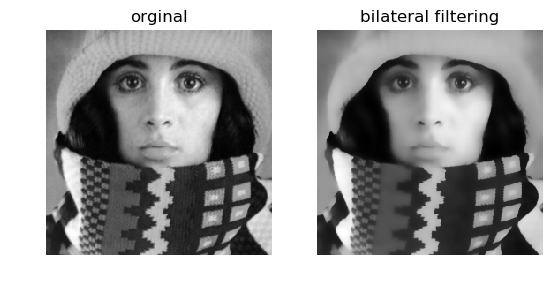
In Gaussian smoothing we take a weighted average of pixel values in the neighborhood. The weights are inversely proportional to the distance from the center of the neighborhood. Besides these spatial weights, the bilateral filter adds a tonal weight such that pixel values that are close to the pixel value in the center are weighted more than pixel values that are more different.
This tonal weighting makes that the bilateral filter is capable of preserving edges (large differences in tonal value) while smoothing in the more flat regions (small tonal differences).
5.4.1. Definition
The bilateral filter starts with linear Gaussian smoothing:
The weight for \(f(\v y)\) equals \(G^s(\v x - \v y)\) and is only dependent on the spatial distance \(\|\v x-\v y\|\). The bilateral filter adds a weighting term that depends on the tonal distance \(f(\v y)-f(\v x)\). This results in:
Observe that because the weights explicitly depend on the image values, we need an explicit normalization such that the ‘sum’ of all weights equals one.
5.4.2. Algorithms
A straightforward algorithm implements the defining equation directly.
def bilateral( f, s, t ):
  def tonaldistsq(fp, fq):
    pass
  def spatialdistsq(p, q):
    pass
  g = empty( f.shape )
  for p in domainIterator(f.shape[:2]):
    t = 0; n = 0
    for q in nbhIterator(f.shape, start, end, p):
      w = exp( -spatialdistsq(p,q)/(2*s**2) ) * exp( -tonaldistsq(f[p],f[q])/(2*t**2) )
      t += f[q] * w
      n += w
    g[p]=t/n
The two functions tonaldistsq and spatialdistsq are to be
specified of course, we leave that as an exercise to the reader. Try
to make tonaldistsq useful with both scalar and color images (the
domain loop already assumes we have a 2D image but leaves room for a
third array dimension: using the f.shape[:2] construction.
This algorithm is slow, very slow… So try it on very small images.
A faster algorithm uses only standard (and thus seperable) Gaussian filters. The disadvantage is that it is only an approximation to the real bilateral filter.
Consider the definition in equation (1). If we set \(f(\v x)\) equal to \(z\) we get a one parameter family of images:
which is called the bilateral stack. Note that now both terms in the fraction for fixed \(z\) are standard convolutions:
where \(f_z\) is the ‘image’: \(f_z(\v y) = G^t(z - f(\v y))\). Now the value of the bilateral filter at position \(\v x\) is given by \(b(\v x, f(\v x))\). So to implement the bilateral filter without error we should calculate \(b(\v x, z)\) for all values of \(z=f(\v x)\) that are in the image.
We may approximate the bilateral filter by calculating \(b(\v x, z)\) only for relatively few values of \(z\) and interpolate to approximate the value for all possible \(z\). From a computational point of view this is efficient because very fast algorithms for Gaussian filtering are known.
In the code below we use a simple linear interpolator. So for a pixel \(\v x\) with value \(f(\v x)\) we only have to consider the two \(z_i\) and \(z_{i+1}\) such that \(z_i\leq f(\v x) \leq z_{i+1}\). Only these two \(z\) values contribute to the interpolated value for \(z=f(\v x)\).
def bilateralInterpolated(f, spatialscale, tonalscale, nslices=10):
    """Bilateral filtering by interpolation in the bilateral stack"""
    zs = linspace(amin(f), amax(f), nslices)
    dz = zs[1] - zs[0]
    g = zeros_like(f)
    for z in zs:
        fz = exp(-(f-z)**2 / (2 * tonalscale**2))
        teller = gaussian_filter(f * fz, spatialscale)
        noemer = gaussian_filter(fz, spatialscale)
        b = teller / noemer
        w = maximum(0, 1-fabs(f-z) / dz)
        g += w * b
    return g
In the loop over all sample values for \(z\) you may recognize the linear interpolation kernel in the expression for \(w\).
5.4.3. Bilateral filtering of color images
The function bilateralInterpolated does work for color images! If
f is a color image then the statement g =
bilateralInterpolated(f, (3,3,0), .1) calculates the scalar
bilateral filter on all three color channels independently. That is
certainly not the best way to do it. It would be better if the tonal
distance were measures in color space to give one scalar value to be
used for all channels. Any meaningfull color distance can be used
here.
Coupling the three channels using a color distance prevents that there is smoothing in say the red channel because the edge between two regions is only visible in the green and blue channel.
We leave it as an exercise to start with a formal definition of a color bilateral filter (and with a straightforward implementation of the definition) and to see whether the color version can be made faster using interpolation in a color bilateral stack (what should that be?).
5.4.4. Theoretical Considerations
The bilateral filter is a simple and elegant extension of the standard Gaussian filter with remarkable properties. For edge preserving smoothing it is the preferred tool for many image processing practitioners.
From a theoretical point of view much more can be said about the bilateral filter:
Robust Local Structure.
It has been shown that the bilateral filter is the first iteration in the robust estimation of the (zero order) local structure. Locally (modelled with a Gaussian aperture) the model is a constant image and instead of using a least squares estimator to find that constant (which would lead to a Gaussian smoothing) a robust estimator is used that can neglect observations that are too far off (compared with the model). For the robust estimator we should iterate the bilateral filter (with the difference that \(f(\v x)\) in eq (1) should be fixed to the original value in all iterations).
Mean Shift
The bilateral filter has also be shown to be related to an estimation procedure called “mean shift analysis”.
Local Mode Estimation.
It can be shown that the bilateral filter is the first step in iteratively finding the local mode in the local image histogram.
Efficient Algorithms
Its remarkable properties lead to the need for more efficient algorithms. The interpolation in the bilateral stack approximation discussed here is only a very simplified version of the bilateral grid based algorithms.