5.3. Percentile Filtering
5.3.1. Definition
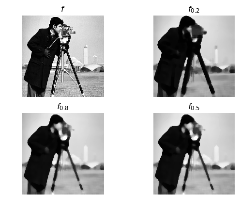
The \(p\)-percentile filter for scalar discrete images is simply defined: in each neighborhood \(\set N_{\v x}\) centered at position \(\v x\) calculate the \(p\)-percentile value of all pixel values in that neighborhood. That percentile value becomes the result of the median filter at position \(\v x\). Repeat this for all neighborhoods, i.e. for all points \(\v x\) in the image and you have implemented the percentile filter.
For an introduction to percentiles (and medians, being the \(0.5\)-percentile) see a section in the Mathematical Tools section.
The above simple definition of the percentile/median filter cannot be readily generalized to work with images defined on a continuous domain, such that every neighborhood will contain an infinite number of points. Therefore we look at a slightly more complex definition.
The \(p\)-percentile filter for scalar images is defined as:
where you should read \(\#\set A\) as the area (or volume depending on the dimensionality of the space) of subset of a continuous domain or as the number of elements in a subset of a discrete domain. And \(f\leq t\) should be interpreted as the subset of the domain of \(f\) where \(f(\v x)\leq t\).
The \(p\)-th percentile is thus that value \(t\) such that \(100 p\) percent of the pixels has a value lower then or equal to \(t\).
The \(p=0.5\) percentile is called the median and the corresponding filter is called the median filter.
Note that the fraction in the above definition is the normalized cumulative histogram of \(f\) restricted to the neighborhood \(\set N_{\v x}\), denoted as \(H_{f|\set N_{\v x}}\), i.e.
5.3.2. Algorithms
For an image defined on a discrete grid (a sampled image) the algorithm is very simple. For every neighborhood \(\set N_{\v x}\) in the image, sort all values \(f(\v y)\) (for \(\v y\in\set N_{\v x}\)) in increasing order and pick the \(p\,\#\set N\)-th value in the ordered sequence.
The following code uses the generic filter function from scipy.ndimage to calculate the p-percentile in a \(K\times K\) neighborhood.
In [1]: from pylab import *

In [2]: from scipy.ndimage import generic_filter

In [3]: def percentileFilter(f, p, K):
   ...:     def pp(v):
   ...:         return percentile(v, 100*p)
   ...:     return generic_filter(f, pp, size=(K,K))
   ...:
This algorithm does not result in a very efficient program. When we move from pixel \((i,j)\) to pixel \((i,j+1)\) the two neighborhoods only differ slightly. Nevertheless all the values in the new neighborhood are sorted from scratch.
The Huang algorithm keeps track of changes in the local histogram while raster scanning the image. When moving from \(\v x_1\) to \(\v x_2\) the values in \(\set N_{\v x_1}\setminus N_{\v x_2}\) must be removed from the histogram and the values in \(\set N_{\v x_2} \setminus \set N_{\v x_1}\) must be added. Given the histogram and the percentile in point \(\v x_1\), the percentile value in the neighborhood centeren at \(\v x_2\) can be easily calculated.
New: integral histograms. Size of the neighborhood is not relevant anymore (we can do all sizes at the same ‘prize’). Disadvantages: a lot of memory needed, and only axis aligned rectangular neighborhoods.
5.3.2.1. Theoretical Considerations
The percentile filter is neither a linear filter nor a morphological filter. It is therefore a filter that is hard to understand from a theoretical point of view.
There has been a lot of effort put into modelling the percentile filter:
Threshold decomposition
For a binary image the percentile filter simply is a linear moving average (using neighborhood \(\set N\)) followed by thresholding at level \(p\,\# \set N\).
It is not hard to show that for every thresholded image \(f\geq t\)…
Mathematical Morphology
A percentile filter can be formulated as the infimum of many dilation. We have:
Unfortunately the set of structuring elements needed grows quite large quickly. Only for very small discrete structuring elements this is of any practical use.
Order Statistics
That part of statistics that deals with ordering measurements and the statistics thereof.